Information Efﬁcient Automatic Object Detection and Segmentation

using Cosegmentation, Similarity based Clustering, and Graph Label

Transfer

Johannes Steffen, Marko Rak, Tim K

onig and Klaus-Dietz T

onnies

Otto von Guericke University Magdeburg, Institute of Simulation and Graphics, Magdeburg, Germany

Keywords:

Object Detection, Object Segmentation, Cosegmentation.

Abstract:

We tackle the problem of unsupervised object cosegmentation combining automatic image selection, coseg-

mentation, and knowledge transfer to yet unlabelled images. Furthermore, we overcome the limitations often

present in state-of-the-art methods in object cosegmentation, namely, high complexity and poor scalability

w.r.t. image set size. Our proposed approach is robust, reasonably fast, and scales linearly w.r.t. the image set

size. We tested our approach on two commonly used cosegmentation data sets and outperformed some of the

state-of-the-art methods using signiﬁcantly less information than possible. Additionally, results indicate the

applicability of our approach on larger image sets.

1 INTRODUCTION

One of the most important problems in image analy-

sis is object segmentation or the slightly more restric-

tive ﬁgure/ ground separation. The task is to label im-

age pixels according to high-level derived meaningful

contents and partitioning it into two distinct but se-

mantically meaningful parts. However, answering the

question whether or not a region of an image is indeed

semantically meaningful for an observer or any other

receiving entity and, hence, belongs to the object in

question, is often a hard task.

Usually, computational models for object segmen-

tation have to be carefully tuned and optimized for

the objects or the object classes that are relevant for

a certain domain. Therefore, when developing a spe-

ciﬁc object segmentation system one tends to consol-

idate object class relevant information and integrate

it, manually or in a supervised learning setting, into a

complex and object class dependent model. Addition-

ally, one can address object segmentation using only

intra image (or single source) information, thus, only

image intrinsic information is used to separate an ob-

ject from the rest of the image (e.g., using edge based

segmentation methods and incorporating spatial co-

herence of an object’s pixels). While this approach

is object class independent as no prior information

about speciﬁc objects is used to derive a model for

segmentation, it is prone to errors since a model for

a general object segmentation is created indirectly.

Thus, general information of how we expect objects

to be represented within an image is introduced either

way. While many approaches learn object class spe-

ciﬁc segmentation and detection models, e.g., with a

ground truth segmented training set representing the

most prominent object features, an interesting ques-

tion to ask is whether it is possible to segment objects

only by example images without any prior knowledge

about the speciﬁc object class.

1.1 Cosegmentation

Given that one does not have any information about

the object in question the idea is to exploit inter im-

age information, thus, aggregating information from

a pair or a set of images, combined with holistic as-

sumptions of how all or at least most of the objects are

represented in images (e.g., spatial coherence, smooth

edges, or shared features of object intrinsic neigh-

bouring regions). Rother et al. (Rother et al., 2006)

were among the ﬁrst trying to enhance object segmen-

tation quality based on exemplary images containing

a common object. They deﬁned cosegmentation as

the task of “segmenting simultaneously the common

parts of an image pair”. Later on, the rather unre-

stricted deﬁnition of the common was reﬁned into the

common object(s) (Vicente et al., 2011).

During the last years, cosegmentation has received

more and more attention in the computer vision and

machine learning community and a vast amount of

different approaches were proposed. Many of the ex-

isting approaches (e.g., (Rother et al., 2006; Vicente

et al., 2010; Mukherjee et al., 2009; Hochbaum and

Singh, 2009)) are based on MRFs (Markov Random

Steffen, J., Rak, M., König, T. and Tönnies, K-D.

Information Efﬁcient Automatic Object Detection and Segmentation using Cosegmentation, Similarity based Clustering, and Graph Label Transfer.

DOI: 10.5220/0005625103970406

In Proceedings of the 5th International Conference on Pattern Recognition Applications and Methods (ICPRAM 2016), pages 397-406

ISBN: 978-989-758-173-1

397

Fields) and do have computationally high complex-

ity. It was soon extended to segmenting commonali-

ties among image sets instead of image pairs. How-

ever, while the ﬁrst approach of segmenting the com-

mon of an image pair implicitly stresses rather hard

assumptions on the image pair used (i.e., the shared

object on both of the images should be “very simi-

lar” to allow for a good matching) the later extension

to image sets allows a greater variety in an object’s

appearance as long as it represented well enough in

the set. Intuitively, one would expect the cosegmen-

tation segmentation quality to increase the more ex-

emplary images of an object are present in the image

set. However, especially in the MRF based solutions

complexity will grow non-linear w.r.t. image set size.

Moreover, given a large image set sharing a common

object it is likely that some subset of it covers the ob-

ject class’ variability well enough. Therefore, when

performing large-scale cosegmentation it is reason-

able to choose exemplary images from the image set,

namely, a subset that covers the class’ variability, in-

stead of performing cosegmentation on the complete

image set as it is done in literature and the MRF based

approaches.

Throughout this work, we will present an ap-

proach to overcome this limitation while maintaining

state of the art performance.

2 RELATED WORK

Most of the MRF based solutions introduce a spe-

cial constraint for foreground similarity and integrate

it within the MRF’s potentials to obtain a matching

across two images instead of segmenting them sep-

arately. There are two key components that differ

in MRF based cosegmentation approaches: 1) the

method used to integrate foreground/ object similar-

ity across the images, and, 2) the optimization pro-

cedure used to minimize the corresponding MRF’s

energy function. Following the notation of (Vicente

et al., 2010), the MRF’s energy function is denoted as

E(x) =

∑

| {z }

unary term

∑

(p,q)

− x

{z }

pairwise term

+λE

global

)

| {z }

similarity term

(1)

where x

and x

denote the pixel labelling x (i.e.,

x ∈ {0,1} for foreground/ background), w

the unary

weight, w

the weight for pairwise labelling smooth-

ness, λ the similarity weight, and h

1,2

being his-

tograms containing (arbitrarily chosen) information

about the foreground of the two images. Hereby, ap-

proaches (e.g., (Rother et al., 2006; Mukherjee et al.,

2009; Hochbaum and Singh, 2009)) differ in the way

how the similarity term E

global

is modelled and what

optimization procedure is used.

Solving the cosegmentation problem using MRFs

is a reasonable approach and yields good results w.r.t.

segmentation quality. However, computational costs

can be rather high. Furthermore, the complexity in-

creases non-linearly with increasing image set size,

e.g., when using the Boykov-Jolly model (Boykov

and Jolly, 2001). Adding a new image to the set of

images the complete Expectation-Maximization algo-

rithm needs to be rerun to cope with new background

and foreground information. Either way, the power of

MRF based solutions lies in the modelling of the class

similarity as well as in the pairwise potentials used for

its formulation and, subsequently, impacts the choice

of how to perform energy minimization and, hence,

performance.

2.1 (Approximative) k - Nearest

Neighbour Approaches

Recently, cosegmentation approaches based on dif-

ferent variants of the so called PatchMatch (PM) al-

gorithm (Barnes et al., 2009; Barnes et al., 2010)

have been proposed. The PM algorithm was not ex-

plicitly developed for cosegmentation tasks but is in-

deed of great beneﬁt since it provides approximative

k Nearest Neighbour Fields (akNNF) within reason-

ably short time. The algorithm avoids the high costs

of ﬁnding exact NNFs using exhaustive minimiza-

tion but rather exploits the fact that it is possible to

ﬁnd suitable matches randomly and propagate those

matches around a certain spatial neighbourhood of the

original match. Regarding object cosegmentation, the

idea to propagate good matches to a certain neigh-

bourhood is indeed plausible since (at least in many

natural images) coherence is believed to be a crucial

property.

Zhang et al. (Zhang et al., 2011) were among

the ﬁrst to propose a labelling approach based on the

PatchMatch algorithm. Therefore, they compute the

dense correspondence ﬁeld over an image pair and

use the resulting akNNF as grounds for label trans-

fer from an already labelled ground truth image set.

Similarly, the work by (Faktor and Irani, 2012; Fak-

tor and Irani, 2013) exploits the PM algorithm to ﬁnd

co-occurring regions across images and then performs

label transfer on the basis of previously computed re-

gion hypothesis called “Soup of Segments”.

Moreover, (Gould and Zhang, 2012) proposed a

new method based on the idea of the PM algorithm

to overcome the limitation that the PM algorithm was

only capable of processing image pairs instead of ar-

ICPRAM 2016 - International Conference on Pattern Recognition Applications and Methods

398

bitrarily sized image sets. Furthermore, they perform

matching on over-segmentations of images instead of

using pixels and modiﬁed the PM algorithm for a

graph based representation. Formally, they deﬁne the

PatchMatchGraph (PMG) over images I as a directed

Graph G(I) = hV,Ei, where nodes u ∈ V represent

patches of image i ∈ I and edges (u,v) ∈ E represent

matches between patches. Using this representation,

they furthermore extended the original idea of pair

correspondence for image sets including more than

two images. Therefore, they exploit the idea that if

image 1 has a good match with 2 and image 2 matches

well with image 3 then it is likely that there is a good

match between images 1 with image 3.

PatchMatch based approaches, in contrast to MRF

based ones, are not image set size sensitive as they

converge reasonably fast and can be extended to cope

with large-scale image sets (Gould and Zhang, 2012;

Gould et al., 2014). However, a drawback of purely

PM based approaches is poor labelling w.r.t. to label

smoothness.

3 METHODS

3.1 Overview

Reviewing related work in the ﬁeld of object coseg-

mentation it becomes evident that existing approaches

often lack practical applicability. Usually, increased

segmentation quality comes at the cost of high

computational complexity (e.g., dense matching ap-

proaches such as in (Rubinstein et al., 2013) or MRF

based approaches mentioned in Section 2) and the

lack of re-usability of previously computed segmenta-

tions, thus, the need to rerun the whole segmentation

procedure for all images when a new image is added

to the cosegmentation set. To overcome this limi-

tation, our approach divides the image set into rea-

sonable clusters that are believed to represent the ob-

ject’s class variability, thus, we propose an approach

to tackle the difﬁculty to (reasonably) balance com-

putational effort while trying to maintain state of the

art performance in object cosegmentation.

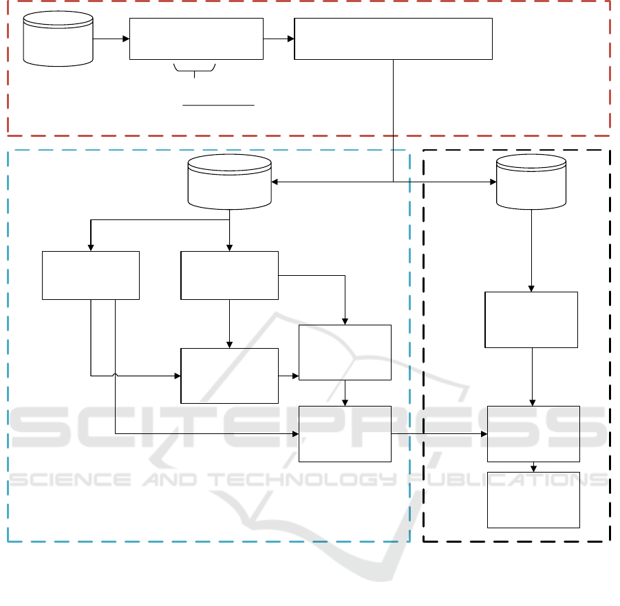
Our approach consists of three subsequent steps:

First, under the assumption that all images in the im-

age set I share a common foreground object, we create

two different sets out of I: 1) a label transferring set

(T ) and 2) a label receiving set (R).

Second, we segment the common foreground ob-

jects in the images of the smaller set T by using inter-

image information and label them as foreground and

the uncommon as background.

Third, we transfer the labels segmented from T to

set R. Figure 1 schematically shows the basic pro-

cessing pipeline including the three steps.

3.2 First Step: Creating the Label

Transferring and the Label

Receiving Set

Given the image set I we cluster all images into k clus-

ters using the k-means algorithm on GIST descriptors

proposed by (Oliva and Torralba, 2001). Since k is

unknown, we repeatedly cluster the images with in-

creasing k (k = 2,3,..., k

max

) 100 times, where k

max

b(0.1 · |I|)c. To select an appropriate k several com-

mon internal validity indices can be evaluated. For

the sake of simplicity, we choose the intra-cluster ho-

mogeneity for selecting k. Therefore, the k with the

smallest resulting error sum of squares averaged over

the k clusters is chosen by a majority voting scheme.

For every k cluster centres resulting from the k-

means clustering we now add the corresponding n

nearest neighbours including the centre to the label

transferring set T . The number of nearest images n is

chosen such that n = max(b(0.3 · |I|)/kc, 5). Finally,

the label receiving set R is generated to contain all

remaining elements of I that are not in the label trans-

ferring set T , i.e., R = I \ T.

Parameter Assumptions. The clustering helps to

ensure that the set from which the labels will later

be transferred covers more object variability than we

might have when T is chosen randomly. Furthermore,

setting n to at least 5 ensures that there are enough

similar images per cluster in T to successfully ap-

ply the common foreground segmentation in the next

step.

3.3 Second Step: Common Foreground

Segmentation

Given the images in T that share a common fore-

ground, we now extract the region-based contrast

(RC) (Cheng et al., 2011) providing a saliency image

quantized into 256 values. We now binarize the image

setting all salient values to 1 and the rest to 0. As a re-

sult we obtain a binarized saliency mask that is used to

regularize the region in this image in which an akNNF

is created using the PatchMatch based method (please

see (Gould and Zhang, 2012; Gould et al., 2014) for

more details) to avoid regions that contain most likely

background information.

Information Efﬁcient Automatic Object Detection and Segmentation using Cosegmentation, Similarity based Clustering, and Graph Label

Transfer

399

 = max(



0.3  #





, 5)

Image Set

(I)

Estimate #Clusters k (extract

n cluster members per k)

RC Saliency Map

Extraction

Create Label Transferring Set T and Label

Receiving Set R out of I (see text)

Transferring Set

(T)

Receiving Set

(R)

Generate Over-

Segmentations

(Regions)

akNNF Generation

on Biggest RC

Mask

Generate Over-

Segmentations

(Regions)

GrabCut

PostPocessing

akNN Graph

Generation for

Label Transfer

Graph Based Label

Transfer

GrabCut Post-

Pocessing

Figure 1: Schematical processing pipeline consisting of the three stages: First Step (red), Second Step (blue), and Third Step

(black).

3.3.1 Over-segmentation

In contrast to (Gould et al., 2014) we decided to use

Ultrametric Contour Maps (UCM) (Arbelaez, 2006)

instead of multi-level superpixel segmentations such

as SLIC (Achanta et al., 2012) to reduce the amount

of regions that need to be processed later on. Hereby,

segments are hierarchically merged following an ul-

trametric inequality equation and, in contrast to SLIC,

purely data-driven merged without any compactness

prior (see Figure 2 for an example).

3.3.2 Region Descriptor

For each region extracted from the UCMs, the same

(and commonly used) features as in (Gould et al.,

2014) were chosen to describe a region’s appearance:

A modiﬁed HOG descriptor by (Felzenszwalb et al.,

2010) with reduced dimensionality (13 dimensions),

concatenated Shannon entropy from the RGB colour

histograms (256 bins each) (3 dimensions), and Lo-

cal Binary Patterns (Ojala et al., 1996; Ojala et al.,

2002) (4 dimensions). We furthermore add the Lo-

cal Self Similarity descriptor proposed by (Shecht-

man and Irani, 2007). Therefore, for each pixel p ∈ I

of the image I a small patch around p is extracted and

compared to the adjacent region within radius r. This

comparison then yields the correlation surface and its

values are transferred into (log)-polar bins. The num-

ber of bins for each histogram is the fourth parame-

ter (the other three being the original patch size, the

size of the neighbouring regions, and the angles con-

trolling the number of circular sectors) to be chosen

ICPRAM 2016 - International Conference on Pattern Recognition Applications and Methods

400

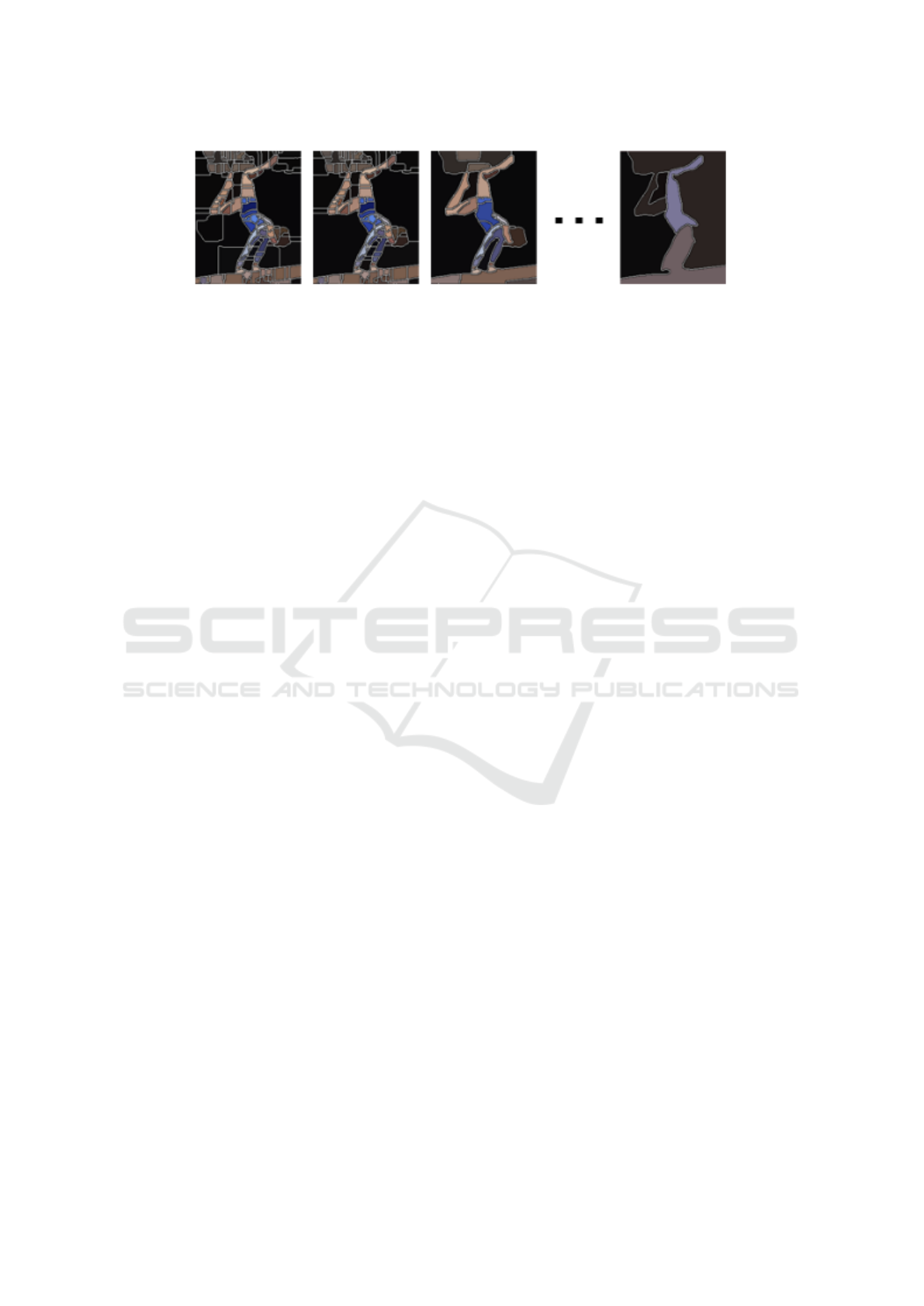
Figure 2: Example visualization of an UCM segmentation: Selected image hierarchy of regions from ﬁne (left) to coarse

(right).

and, because we are binning in log-polar coordinates,

it represents the number of evenly spaced radii in log-

polar domain. To form the descriptor, the highest cor-

relation in each of the obtained histograms is chosen.

Here, we use the standard parameters using 4 bins, 4

circular sectors, and patch size of 5x5 yielding a 16-

dimensional vector.

As in (Gould et al., 2014), after concatenating the

feature vectors, the region descriptor is enriched with

the location (x and y) of the region’s centroid as well

as its respective area. Moreover, to account for spa-

tial neighbours of the region, the mean and standard

deviation of the features of the four neighbouring re-

gions are appended. Finally, averaging the features

across and taking the standard deviation over all pix-

els within the region, yields the overall descriptor (see

(Gould et al., 2014) for further details).

3.3.3 Creating the Label Transfer Graph

Creating the label transfer graph closely follows the

work of (Gould et al., 2014) to whom we refer for a

detailed description and a very good implementation

(Gould, 2012) of the PatchMatch based Graph Label

Transfer. Nonetheless, we will brieﬂy explain the key

concept for the sake of clarity:

Each image in T is now regularized by its corre-

sponding RC saliency map and a hierarchical over-

segmentation using UCMs is extracted. Furthermore,

for each resulting region in each UCM layer, a region

descriptor is computed as described above. Follow-

ing the notation of (Gould et al., 2014), the images

in T are now represented as a graph G(V,E), where

the nodes u ∈ V represent UCM regions, the edges

(u,v) ∈ E represent a connection/ match between two

regions, and x

the feature vector associated with re-

gion u.

The goal is to ﬁnd similarities, thus, to ﬁnd the k

nearest neighbours for each region. I.e., the following

minimization problem has to be solved (Gould et al.,

2014)

minimize

∑

(u,v)∈E

d(u,v) (2)

subject to ∀u ∈ V : deg(u) = k

∀(u,v) ∈ E : image(u) 6= image(v)

∀(u,v),(u,w) ∈ E : image(v) 6= image(w),

where d(u,v) denotes the distance between two

regions described by their corresponding feature vec-

tors.

The ﬁrst constraint hereby enforces that k nearest

neighbours are computed for each region, the second

constraint forbids edges between regions of the same

image, and the last constraint is used to enforce solu-

tion diversity, that is, each of the k nearest neighbours

is located on a different image. Please note, that the

aforementioned parameter k for the number of near-

est neighbours is different from the parameter k of the

clustering step.

Since it is costly to perform an optimization of

Equation 2, instead of computing exact matches,

the problem is relaxed to ﬁnd (approximate) nearest

neighbours which is done by the modiﬁed version of

the generalized PatchMatch algorithm introduced by

(Gould and Zhang, 2012).

To provide an overview of the steps involved in

ﬁnding an approximative solution for Equation 2 the

basic idea of each step is outlined below. A more de-

tailed explanation can be found in the original work of

(Gould and Zhang, 2012). In our case, we are inter-

ested in ﬁnding the 10 (approximative) nearest neigh-

bours for each given region due to empirical evalua-

tions given by (Gould et al., 2014).

• Initialization: During the initialization phase of

the PM algorithm, a random Nearest Neighbour

Field is set up, thus, the respective regions are

given random correspondence assignments that

account for the constraints in Equation 2. This

step is only performed once and the following

steps are repeated until some halting criteria is

met.

• Propagation: Given good assignments from the

initialization step or from the previous iteration,

Information Efﬁcient Automatic Object Detection and Segmentation using Cosegmentation, Similarity based Clustering, and Graph Label

Transfer

401

the algorithm will propagate these assignments

to neighbouring pixels if the region is coherent.

That is, on even iterations the algorithm will try

to propagate the assignment to the left and top of

the respective pixel in an attempt to improve the

respective neighbouring matches and on odd iter-

ations to the right and bottom. However, the new

assignment will only be propagated if the error is

smaller than the one previously assigned.

• Decaying Search: Designed to avoid getting stuck

in locally optimal solutions, in this step, given a

(good) match between two nodes (u,v), the algo-

rithm randomly samples patches around an expo-

nentially decaying neighbourhood of v to eventu-

ally ﬁnd better matches. Here, the number of iter-

ations is set to 500.

• Forward Enrichment: This step is designed to

propagate (good) matches along the image set.

The idea was already described above, thus, given

(good) matches (u,v) and (v,w) the edge (u,w) is

believed to be a (good) match as well.

• Local Search: During this step, the algorithm tries

to ﬁnd a better matching node v

in the neighbour-

hood of v given a (good) match (u,v).

• Inverse Enrichment: Originally introduced by the

PatchMatch extension of (Barnes et al., 2010)

which is based on the idea that, given a (good)

match (w, u) it is likely that there is also a good

match (u,w). Thus, if an edge (w,u) is added then

(u,w) is added as well if not already present.

• Exhaustive Search: This can be used as an ini-

tialization for the matches. Therefore, for a few

patches of an image it searches exhaustively for k

nearest neighbours of this patch (in different im-

ages). Though this step is rather expensive, it only

has to be done for a small number of patches so

that the move-steps above are provided with a suf-

ﬁciently good initialization and, hence, will not

get stuck in far from optimal solutions. Here, the

number of iterations is set to 500.

• Halting Criteria: Iterating through the propaga-

tion and search step, the algorithm halts either

after (soft) convergence, thus, if no assignments

change over a period of some iterations or after a

ﬁx number of iterations.

After the approximation has converged we pro-

ceed to extract the binary masks based on the RC

saliency maps with lowest matching costs and deﬁne

them as the common foreground.

Finally, to obtain the overall object cosegmenta-

tions of the images in T we apply GrabCut (Rother

et al., 2004) based on three inputs for model genera-

tion for each image in T: The foreground model taken

from the binary mask with lowest matching costs, the

background model taken from the inverted largest bi-

narized RC mask (mentioned in the ﬁrst paragraph of

this section), and a “possible” foreground model for

all other pixels that are neither labelled background

nor foreground. As a result we now have a com-

mon foreground (object) / background segmentation

for each image in T .

After the graph is set up, a metric learning ap-

proach is performed to estimate the metric that min-

imizes the distance between UCM regions sharing a

common label while maintaining large distance for re-

gions that do not share a common label (Gould et al.,

2014). This is done exhaustively until convergence.

3.4 Third Step: Label Transfer

Similarly to the previous steps in 3.3.1, 3.3.2, and

3.3.3 we set up a second graph for the label receiving

set R, thus, we perform the UCM over-segmentation

and compute the feature vector as described above for

each image in R. Note that in this case we do not need

to extract the saliency maps, since we are now inter-

ested to transfer the label knowledge from set T to the

new image data in R.

To do this, the approximative optimization of

Equation 2 is now repeated after both graphs (the la-

bel transferring and the label receiving) are merged

with the additional restriction, that edges between re-

gions of the label receiving images are forbidden.

After the approximation has converged, the labels

are then transferred by a majority vote of the akNNs,

thus, for every pixel in every image of R all found

nearest neighbours of its enclosing UCM regions are

evaluated and, if the majority of its regions are la-

belled as common foreground, the corresponding la-

bel (1) is assigned to this pixel and vice versa.

Processing. To handle non-smooth labelling when

using UCMs instead of superpixels, again, a GrabCut

is used to smooth the results.

4 RESULTS AND EVALUATION

Contrarily to other cosegmentation approaches we re-

frained from testing our approach against the com-

monly used iCoseg dataset (Batra et al., 2010) since

on average, there are only around 17 images per class

which, due to the small set size, we consider inappro-

priate for our approach. More importantly, our ap-

proach tries to ﬁnd exemplary images that describe

ICPRAM 2016 - International Conference on Pattern Recognition Applications and Methods

402

Table 1: Tabular comparison of our method to the related work on MSRC using established quality measures, method Average

Precision (left) and Jaccard Coefﬁcient (right). Methods with best performance per class are marked bold.

MSRC

Average Precision Jaccard Coefﬁcient

Joulin2010 Joulin2012 Rubinstein2013 Ours Joulin2010 Joulin2012 Rubinstein2013 Ours

bike .64 .68 .78 .66 .39 .46 .54 .18

bird .67 .74 .94 .87 .28 .37 .67 .56

car .77 .79 .84 .82 .58 .62 .67 .58

cat .63 .75 .90 .85 .34 .45 .66 .53

chair .75 .68 .88 .83 .46 .40 .62 .52

cow .78 .83 .94 .94 .53 .61 .79 .76

dog .76 .76 .90 .81 .47 .47 .67 .41

face .80 .84 .82 .81 .56 .69 .58 .54

ﬂower .67 .66 .86 .85 .47 .46 .71 .69

house .62 .58 .87 .87 .43 .41 .73 .67

plane .50 .53 .87 .86 .18 .23 .57 .51

sheep .88 .90 .92 .92 .68 .72 .79 .77

sign .79 .75 .93 .88 .56 .52 .82 .68

tree .67 .81 .83 .79 .40 .69 .70 .60

Avg. .71 .74 .88 .84 .45 .51 .68 .57

Table 2: Tabular comparison of our method to the related work on BigSet using established quality measures, namely Average

Precision (left) and Jaccard Coefﬁcient (right). Methods with best performance per class are marked bold.

BigSet

Average Precision Jaccard Coefﬁcient

Joulin2010 Joulin2012 Rubinstein2013 Ours Joulin2010 Joulin2012 Rubinstein2013 Ours

Airplane .59 .59 .88 .92 .37 .35 .56 .60

Car .64 .64 .85 .86 .30 .30 .64 .65

Horse .49 .47 .83 .84 .15 .12 .52 .51

Avg. .57 .57 .85 .87 .28 .25 .57 .59

the object class’ variability reasonably well but on the

iCoseg dataset most of the images share the very same

object with sometimes even the same backgrounds

and viewing conditions. However, we tested our ap-

proach on a compiled version of the MSRC (Microsoft

Research Cambridge) dataset by (Rubinstein et al.,

2013). This compiled version of MSRC consists of

14 classes containing around 30 images each and was

also benchmarked by (Rubinstein et al., 2013) against

the methods of (Joulin et al., 2010) and (Joulin et al.,

2012). It has to be stressed that even on this dataset

there are way too few different object images to rep-

resent the class variability well.

A more appropriate dataset for our case of object

cosegmentation using only a few images to represent

a whole object class is BigSet provided by (Rubinstein

et al., 2013). The set includes three classes each con-

taining 100 images retrieved by querying an image

search using Microsoft’s search engine Bing. This set

is particularly interesting since its corresponding ob-

ject instances are highly diverse. Therefore, we hy-

pothesized that we can compete with the current state

of the art of (Rubinstein et al., 2013).

We measured the segmentation quality according

to the related work, i.e. using the average precision

(although it is a ﬂawed measure on this kind of prob-

lems due to foreground/ background imbalance) as

well as the Jaccard Coefﬁcient.

As can be seen in Table 1 our method performed

worse than (Rubinstein et al., 2013) but outperformed

(Joulin et al., 2010; Joulin et al., 2012) in almost all

classes. The results are not surprising because we im-

plicitly assume some kind of object appearance re-

dundancy when extracting the n neighbours out of

k clusters for cosegmentation, and often, 30 images

are insufﬁcient to capture an object class’ variability.

However, our approach performed reasonably well

and in the magnitude of related work.

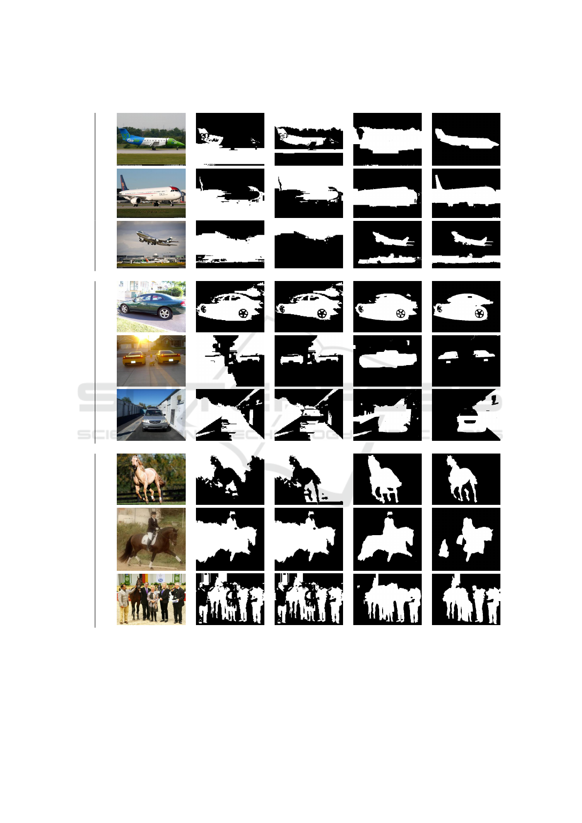
Table 2 shows results for the BigSet. Although the

method by (Rubinstein et al., 2013) clearly outper-

formed our approach on MSRC we managed to get

slightly better averaged results on this data set. For

the Airplane100 class our approach found k = 7 clus-

ters and extracted n = 5 images each. Thus, |T | = 35

images/ objects provided enough (and the right) infor-

mation to label the rest of the images appropriately.

For Car100 |T | = 45 with k = 9 and n = 5 were au-

tomatically found and used to perform label transfer.

Finally, for Horse100 the algorithm only found k = 3

clusters with n = 9 images each, a fact we do not be-

Information Efﬁcient Automatic Object Detection and Segmentation using Cosegmentation, Similarity based Clustering, and Graph Label

Transfer

403

BigSet

Image Joulin2010 Joulin2012 Rubinstein2013 Ours

Airplane

Good

MediumBad

Car

Good

MediumBad

Horse

Good

MediumBad

Figure 3: Visual comparison of our approach to the related work on a selection of images from BigSet. For each class, an

image with bad, medium, and good result quality was selected. The selected images reﬂect the ﬁrst, second, and third quantile

of Jaccard Coefﬁcients of our method on each particular class.

lieve corresponds well with the visual object variabil-

ity seen in the Horse100 set.

For visual comparison Figure 3 shows some ex-

ample segmentations compared to (Rubinstein et al.,

2013; Joulin et al., 2012; Joulin et al., 2010).

ICPRAM 2016 - International Conference on Pattern Recognition Applications and Methods

404

5 CONCLUSION AND REMARKS

In this work we have presented an unsupervised ob-

ject cosegmentation approach that overcomes certain

limitations that other state-of-the-art methods exhibit.

We have shown, that most of the current methods

based on MRFs or dense (exact) correspondences are

limited by the fact that they cannot leverage knowl-

edge to new images that need to be segmented.

Our approach is capable of object cosegmenta-

tion yielding state-of-the-art performance while be-

ing scalable to larger image sets and using less in-

formation to infer labels on yet unseen images. Our

results indicate that carefully choosing representative

object class clusters that account for the object class’

intrinsic variability can compensate for information

that needs to be present when cosegmentation is per-

formed over a whole image set. We do note, however,

that the current choice of the transfer set T is based

on simple assumptions about global image statistics

that might not work for images on which the common

foreground is among other objects or on very cluttered

background. Furthermore, the results are promising

and we plan to test our approach on larger image sets

incorporating dynamic updating of the transfer set T

when images are added to the set one after the other.

ACKNOWLEDGEMENTS

This research was partially funded by the project Vi-

sual Analytics in Public Health (TO 166/13-2), which

is part of the Priority Program 1335: Scalable Visual

Analytics of the German Research Foundation.

REFERENCES

Achanta, R., Shaji, A., Smith, K., Lucchi, A., Fua, P., and

usstrunk, S. (2012). Slic superpixels compared to

state-of-the-art superpixel methods. IEEE transac-

tions on pattern analysis and machine intelligence,

34(11):2274–2282.

Arbelaez, P. (2006). Boundary extraction in natural images

using ultrametric contour maps. In 2006 Conference

on Computer Vision and Pattern Recognition Work-

shop (CVPRW’06), page 182.

Barnes, C., Shechtman, E., Finkelstein, A., and Goldman,

D. B. (2009). Patchmatch: A randomized corre-

spondence algorithm for structural image editing. In

Funkhouser, T. and Hoppe, H., editors, ACM SIG-

GRAPH 2009 papers, page 1.

Barnes, C., Shechtman, E., Goldman, D. B., and Finkel-

stein, A. (2010). The generalized patchmatch corre-

spondence algorithm. In Daniilidis, K., Maragos, P.,

and Paragios, N., editors, Computer Vision – ECCV

2010, volume 6313 of Lecture Notes in Computer

Science, pages 29–43. Springer Berlin Heidelberg,

Berlin, Heidelberg.

Batra, D., Kowdle, A., Parikh, D., Luo, J., and Chen, T.

(2010). icoseg: Interactive co-segmentation with in-

telligent scribble guidance. In 2010 IEEE Conference

on Computer Vision and Pattern Recognition (CVPR),

pages 3169–3176.

Boykov, Y. Y. and Jolly, M.-P. (2001). Interactive graph

cuts for optimal boundary & region segmentation of

objects in n-d images. In Eighth IEEE International

Conference on Computer Vision, pages 105–112.

Cheng, M.-M., Zhang, G.-X., Mitra, N. J., Huang, X., and

Hu, S.-M. (2011). Global contrast based salient re-

gion detection. In 2011 IEEE Conference on Com-

puter Vision and Pattern Recognition (CVPR), pages

409–416.

Faktor, A. and Irani, M. (2012). “clustering by composi-

tion” – unsupervised discovery of image categories.

In Daniilidis, K., Maragos, P., and Paragios, N., edi-

tors, Computer Vision – ECCV 2012, volume 7578 of

Lecture Notes in Computer Science, pages 474–487.

Springer Berlin Heidelberg, Berlin, Heidelberg.

Faktor, A. and Irani, M. (2013). Co-segmentation by com-

position. In 2013 IEEE International Conference on

Computer Vision (ICCV), pages 1297–1304.

Felzenszwalb, P. F., Girshick, R. B., McAllester, D., and

Ramanan, D. (2010). Object detection with discrim-

inatively trained part-based models. Pattern Analy-

sis and Machine Intelligence, IEEE Transactions on,

32(9):1627–1645.

Gould, S. (2012). Darwin: A framework for machine learn-

ing and computer vision research and development.

Journal of Machine Learning Research, 13(1):3533–

3537.

Gould, S. and Zhang, Y. (2012). Patchmatchgraph: Build-

ing a graph of dense patch correspondences for label

transfer. In Daniilidis, K., Maragos, P., and Paragios,

N., editors, Computer Vision – ECCV 2012, volume

7576 of Lecture Notes in Computer Science, pages

439–452. Springer Berlin Heidelberg, Berlin, Heidel-

berg.

Gould, S., Zhao, J., He, X., and Zhang, Y. (2014). Super-

pixel graph label transfer with learned distance metric.

In Fleet, D., Pajdla, T., Schiele, B., and Tuytelaars, T.,

editors, Computer Vision – ECCV 2014, volume 8689

of Lecture Notes in Computer Science, pages 632–

647. Springer International Publishing, Cham.

Hochbaum, D. S. and Singh, V. (2009). An efﬁcient al-

gorithm for co-segmentation. In 2009 IEEE 12th In-

ternational Conference on Computer Vision (ICCV),

pages 269–276.

Joulin, A., Bach, F., and Ponce, J. (2010). Discriminative

clustering for image co-segmentation. In 2010 IEEE

Conference on Computer Vision and Pattern Recogni-

tion (CVPR), pages 1943–1950.

Joulin, A., Bach, F., and Ponce, J. (2012). Multi-class

cosegmentation. In 2012 IEEE Conference on Com-

puter Vision and Pattern Recognition (CVPR), pages

542–549.

Information Efﬁcient Automatic Object Detection and Segmentation using Cosegmentation, Similarity based Clustering, and Graph Label

Transfer

405

Mukherjee, L., Singh, V., and Dyer, C. R. (2009). Half-

integrality based algorithms for cosegmentation of im-

ages. In 2009 IEEE Computer Society Conference on

Computer Vision and Pattern Recognition Workshops

(CVPR Workshops), pages 2028–2035.

Ojala, T., Pietik

ainen, M., and Harwood, D. (1996). A com-

parative study of texture measures with classiﬁcation

based on featured distributions. Pattern Recognition,

29(1):51–59.

Ojala, T., Pietikainen, M., and Maenpaa, T. (2002). Mul-

tiresolution gray-scale and rotation invariant texture

classiﬁcation with local binary patterns. IEEE Trans-

actions on Pattern Analysis and Machine Intelligence,

24(7):971–987.

Oliva, A. and Torralba, A. (2001). Modeling the shape

of the scene: A holistic representation of the spatial

envelope. International Journal of Computer Vision,

42(3):145–175.

Rother, C., Kolmogorov, V., and Blake, A. (2004). Grabcut

-interactive foreground extraction using iterated graph

cuts. ACM Transactions on Graphics (SIGGRAPH).

Rother, C., Minka, T., Blake, A., and Kolmogorov, V.

(2006). Cosegmentation of image pairs by histogram

matching - incorporating a global constraint into mrfs.

In Computer Vision and Pattern Recognition, 2006

IEEE Computer Society Conference on, volume 1,

pages 993–1000.

Rubinstein, M., Joulin, A., Kopf, J., and Liu, C. (2013). Un-

supervised joint object discovery and segmentation in

internet images. In 2013 IEEE Conference on Com-

puter Vision and Pattern Recognition (CVPR), pages

1939–1946.

Shechtman, E. and Irani, M. (2007). Matching local self-

similarities across images and videos. In 2007 IEEE

Conference on Computer Vision and Pattern Recogni-

tion, pages 1–8.

Vicente, S., Kolmogorov, V., and Rother, C. (2010). Coseg-

mentation revisited: Models and optimization. In

Daniilidis, K., Maragos, P., and Paragios, N., edi-

tors, Computer Vision – ECCV 2010, volume 6312 of

Lecture Notes in Computer Science, pages 465–479.

Springer Berlin Heidelberg, Berlin, Heidelberg.

Vicente, S., Rother, C., and Kolmogorov, V. (2011). Object

cosegmentation. In 2011 IEEE Conference on Com-

puter Vision and Pattern Recognition (CVPR), pages

2217–2224.

Zhang, H., Fang, T., Chen, X., Zhao, Q., and Quan, L.

(2011). Partial similarity based nonparametric scene

parsing in certain environment. In 2011 IEEE Con-

ference on Computer Vision and Pattern Recognition

(CVPR), pages 2241–2248.

ICPRAM 2016 - International Conference on Pattern Recognition Applications and Methods

406