A Vehicular Traffic Simulator Model for Evaluating Electrical
Vehicles (EVs) Performances in a Configurable Mobility Scenario
Pierfrancesco Raimondo, Amilcare Francesco Santamaria, Floriano De Rango and Antonio Bosco
Unical, Via Pietro Bucci, Rende, Italy
Keywords:
Simulation, Vehicular, Energy Consumptions, Electric Vehicle, Mobility Model.
Abstract:
Nowadays Electrical Mobility (EM) is one of the most interesting topics in vehicular environment. With the
increasing adoption of EV an appropriate management of hybrid traffic could be a key factor to drastically
reduce environmental pollution and to enhance road safety. EVs were slowly becoming a reality in everyday
life. A novel mobility model which takes into account their characteristics become necessary for describing
the key factors that influence EM and its performances. Moreover, it is important to build a real world close
scenario by using a novel ad-hoc simulator that implements modules which are able to capture EV behaviors.
Therefore, remarkable contributions to the mobility model introduced in the simulator are: a slope factor that
influence users’ speed and behavior as well as vehicle consumption, a Kinetic Energy Recovery System (KERS)
emulation for EV to better simulate vehicles’ battery life and integrated module for communication issues
which will be able to allow Vehicular Ad-Hoc Network (VANET) protocol integration. In this way, a deep
analysis on different vehicles distribution ratio has been done as well as their impact on the overall scenario.
Results are shown in the dedicated section.
1 INTRODUCTION
According to recent researches the number of EV sold
in the last years has increased of 200%. One of the
most adverse factor for the users against the use of
EV is the difficulty of finding charge stations inside
the city, battery duration and the significant amount of
time that a full-charge needs. The number and posi-
tion of these kinds of vehicle can have a great impact
on the traffic dynamics and should be taken into ac-
count. This will allow us to better understand distribu-
tion of traffic flows and their dynamics. To better an-
alyze these kinds of scenario an ad-hoc simulator has
been written in the Java language. Classic vehicular
simulators have been improved and refined for many
years but they do not take into account some charac-
teristics that highly influence EVs and the use of their
battery packs to move. For these reasons, in this pa-
per we propose some enhancement to the simulation
model to better depict new scenarios with a remark-
able number of vehicles that use electricity to move
in the urban and sub-urban areas. One of the fac-
tors that most influence battery lifetime of vehicles is
the road gradient. This factor does not only influence
EV but also fuel engine vehicle and should be taken
into account when simulating vehicles flows inside an
urban scenario. Also some improvement to extend
EV battery lifetime has been developed through years
and have been adopted lately by automotive compa-
nies. One big improvement is the use of regenerative
braking that is capable of transforming part of the ki-
netic energy that is dissipated as heat in reusable en-
ergy that can replenish vehicle battery. In this simula-
tor some innovative concepts have been developed to
have more accurate results:
• Influence of slope on energy consumptions
• A KERS module for regenerative braking
The slope module takes into account street slope cal-
culating a slope coefficient that influences vehicles
speed and consumption as well as driver behavior.
The KERS module is used to better simulate vehi-
cles battery life. Every time a vehicle with KERS
equipped brakes some of the kinetic energy of the de-
celeration is recovered end reused to increase battery
life span.
This work is organized as follows:
• In Section II a brief introduction and the status of
the art on simulating vehicles are presented point-
ing out major differences
• Section III consists of a detailed description of the
simulator. The mobility model used in simula-
198
Raimondo, P., Santamaria, A., Rango, F. and Bosco, A.
A Vehicular Traffic Simulator Model for Evaluating Electrical Vehicle Performances in a Configurable Mobility Scenario.
DOI: 10.5220/0006919301980205
In Proceedings of 8th International Conference on Simulation and Modeling Methodologies, Technologies and Applications (SIMULTECH 2018), pages 198-205
ISBN: 978-989-758-323-0
Copyright © 2018 by SCITEPRESS – Science and Technology Publications, Lda. All rights reserved

tions is explained exhaustively together with the
new modules that take into account the street gra-
dient and the regenerative braking.
• In Section IV simulation results are presented
• In Section V Conclusions and future activities are
presented at last.
2 RELATED WORKS
Lately one of the most requested features for a traf-
fic urban simulator is the possibility to work on real
maps. Authors in (Bieker et al., 2015) developed real
traffic simulation scenarios with Simulation of Urban
MObility (SUMO) for the city of Bologna. They mod-
eled the road networks, traffic lights and also addi-
tional traffic infrastructure. Moreover, traffic simula-
tor is very important to evaluate other communication
issues such as protocol and multimedia data dissemi-
nation avoiding resources wastages as shown in (Kur-
mis et al., 2015; Kurmis et al., 2017; Fazio et al.,
2017). Vehicular simulators permit to test massive
mobility scenarios where both traffic and network is-
sues are analyzed for finding suitable solutions. In
the VANET environment there are several problems to
take under consideration. One of the most important
is represented by interferences. In (Fazio et al., 2011;
Fazio et al., 2012) works author propose a mechanism
for disseminate data tackling interferences issues. In
(Waraich et al., 2015), a new microscopic approach to
traffic simulation is proposed in which a multi-agent
platform is used and several ways to improve overall
performance are presented. Authors of (Zhou et al.,
2015) propose a mesoscopic dynamic traffic simula-
tor with the introduction of consumption evaluation to
evaluate vehicle emission/fuel consumption impact.
A study on how cumulative accelerations can have
a considerable impact on consumption and consecu-
tively on emissions si carried out in (Hemmerle et al.,
2016). In this work the authors show how synchro-
nized flow patterns have a great impact on the over-
all emissions inside cities. A deep investigation of
the different phases of traffic models has been car-
ried out in (Knospe et al., 2000). Authors focused
on how model free-flow, synchronized, and stop-and-
go situations that are present in real traffic. In (Maia
et al., 2011) the authors propose an electric vehicle
simulator based on SUMO to better investigate the
issue of energy consumption of EV. They extended
the classical two-dimensional simulator modeling the
altitude of the streets and transforming in this way
SUMO into a three-dimensional simulator. A descrip-
tion of the development and modules of SUMO is
present in (Krajzewicz et al., 2012). In this paper au-
thors describe the packages composing the simulator
as well as the major applications categorized by re-
search topic and by example. Authors of (Olascuaga
et al., 2015) explored like us the impact of this new al-
ternative technology on users’ driving patterns and on
the energy consumption of vehicles. They did not take
into account the influence of street gradient and re-
generative braking on batteries duration. In (Bedogni
et al., 2014) authors developed and algorithm to plan
the route of an EV taking into account the overhead
to reach the charging stations along the way towards
the destination. However their algorithm do not con-
sider the status of traffic flows inside the moving area
and consequently neither the energy consumed due to
other vehicle interactions
3 SIMULATOR
Nowadays models used in simulators are very precise
and accurate in describing urban scenarios of moving
vehicles. Mobility models are able to describe in a re-
alistic way how vehicles move inside the city. Unfor-
tunately these models do not take into account some
key factors that can influence considerably EV. These
factors can heavily influence the battery lifetime of
this kind of vehicles. The energy consumption of an
electric engine changes depending on a multitude of
factors. One of the most important is the gradient of
the street in which vehicles move. The slope factor
also influence the consumption of fuel engines but af-
fect in a really particular way the energy consumption
of batteries of moving vehicles. For these reasons,
to improve the performances of these kinds of vehi-
cle some countermeasures needs to be developed to
tackle an excessive energy consumption. One of the
most used technique, derived also from motor racing,
is the regenerative braking. Using this technique the
kinetic energy of braking is partially transformed in
electrical energy to refill the engine battery. The pos-
sibility to evaluate novel solutions in a simulated and
controlled environment may help to reduce troubles
in applying new solution in the real world. In next
sections the overall architecture of the simulator will
be presented as well as a description of the innovative
modules that have been introduced.
3.1 Architecture
The proposed simulator framework is based on Dis-
crete Event Simulation (DES) principles and it is com-
posed of several modules which are herein summa-
rized:
A Vehicular Traffic Simulator Model for Evaluating Electrical Vehicle Performances in a Configurable Mobility Scenario
199

• Scheduler/Dispatcher
• Map module
• Mobility module
• Consumption Module
• Slope Module
• Vehicular Module
3.1.1 Scheduler
The scheduler is the heart of the simulator and has
the task to elaborate the events in chronological or-
der. Each created event is pushed into the buffer of
the scheduler in a time-sorted way. The events ex-
tracted from the queue are then analyzed and passed
with Java reflection to the recipient. Every recipient
has a method to manage the message
3.1.2 Map Module
The map module takes care of building a map where
vehicles move. The map is represented by an ori-
ented graph that derives directly from the represen-
tations of real maps that can be found on Open Street
Map (OSM) (osm, 2018). For this purpose an eXtensi-
ble Markup Language (XML) parser has been devel-
oped that parse the structure of the file and build the
graph representation used inside the simulations. In-
formation about streets slope is derived instead from
the Google Maps API.
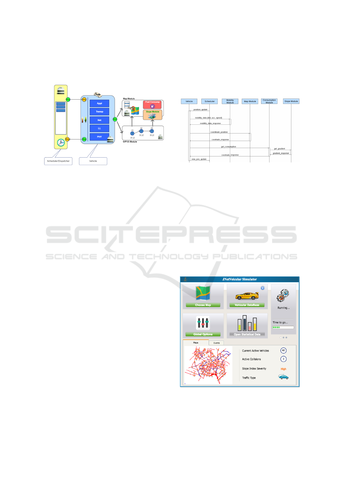
Figure 1: Framework integration for Map modules.
This information is encapsulated inside the map
graph as a property of the edges. The map is also
divided in zones with an altitude coefficient. This co-
efficient is used for consumption estimation. In Fig-
ure 1 the procedures needed for building the map area
used in the simulation are shown. OSM allows users
to download an XML file representing all the inter-
esting features of a chosen area. The XML extracts
the topology of the map building a representative map
graph of the interested area. For each node a call to
the Google Maps API is carried out in order to col-
lect the altitude of each node. The slope is evaluated
and stored as attribute of the edge that connect two
adjacent nodes. Figure 2 shows the map area as result
of the whole process started from the acquisition of
OSM data related to a San Francisco sub-area.
3.1.3 Slope Module
One of the most important simulator enhancement is
the introduction of the slope factor achieve by the
parsing of altitude information. In order to gather in-
formation about street height a software interface with
Google Maps API web services (map, 2018) has been
developed. Due to the limitations use of the Google
Maps Api we had to minimize the number of requests
through altimetry data caching. To collect these in-
formation it is necessary to make a RESTful request
to the serve specifying latitude and longitude coor-
dinates of the point of interest. In addition to node
height also an Altimetric Coefficient (AC) has been
introduced. This coefficient measure the slope factor
of an area given the slope of the segments that are in-
side it. The AC of an area is calculated:
AC =
n
∑
i=1
(segment length
i
/total length) ∗slope
i
(1)
Where n is the number of area segments. Using this
coefficient it is possible to divide areas in three differ-
ent classes:
• low class: areas with AC between 0 and 2
• medium class: areas with AC between 2 and 5
• high class: areas with AC more than 5
3.1.4 Energy Consumption
In order to explain how we introduced inside the sim-
ulator the regenerative braking module we need to
show how we manage the energy consumption of ve-
hicles. Energy consumption into our simulator takes
into account:
• vehicle instantaneous speed
• vehicle instantaneous acceleration (a)
• street gradient angle coming from AC
• battery energy load expressed in kW h
Regarding vehicles’ movement we take into account
three forms of energy depletion:
SIMULTECH 2018 - 8th International Conference on Simulation and Modeling Methodologies, Technologies and Applications
200

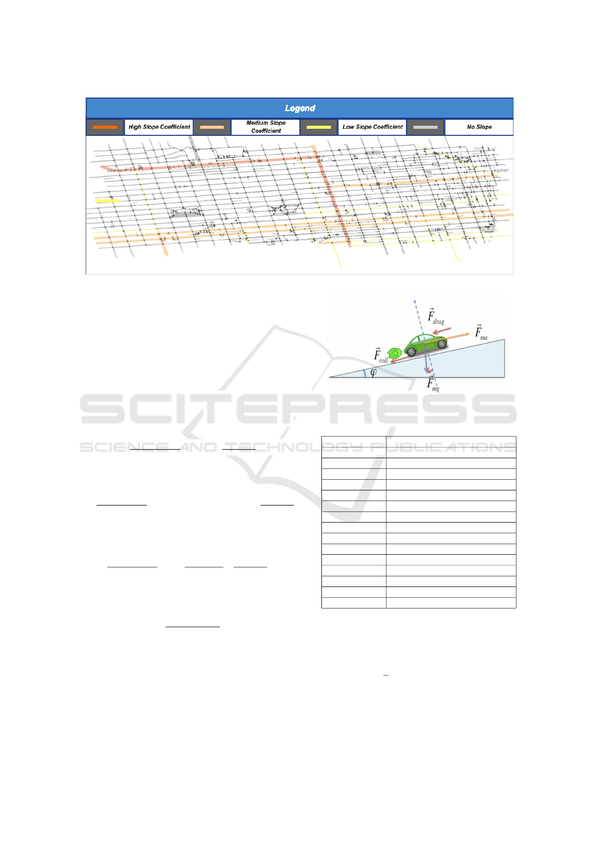
Figure 2: San Francisco graph representation.
• W
v
is the work necessary to move the vehicle
• W
t
is the work necessary to overcome tires friction
• W
a
is the work necessary to overcome air friction
Taking in consideration
m ∗ a = F − m ∗ g ∗ sinϕ (2)
The necessary force to move the vehicle taking into
account the street gradient is
F = m ∗ (a + g ∗ sinϕ) (3)
and its work is
W
v
=
1
E f f iciency
v
∗ ∆t ∗ F ∗
V +V
old
2
(4)
The mass vehicle m is known as well as its efficiency.
The work necessary to withstand tires friction is:
W
t
=
1
E f f iciency
v
∗∆t ∗(m∗g∗cosα∗cRoll)∗
V +V
old
2
(5)
Where cRoll is the friction coefficient of tires. The
work necessary to withstand air friction is :
W
a
=
1
E f f iciency
v
∗ ∆t ∗
ρ ∗ cDrag
2
∗
V +V
old
2
(6)
The model used is shown in 3.
And so energy depletion model can be expressed
like:
E
d
=
W
v
+W
t
+W
a
3600000
(7)
that is subctracted to the energy inside vehicle battery.
3.1.5 Energy Recovery Brake
Part of the energy that is dissipated through air heat-
ing below the brakes can be recovered through a par-
ticular device that very often is used in EV environ-
ment called KERS. To add this device effect to the
Figure 3: energy depletion model.
Table 1: Table of Symbols.
Symbol Name Description
W
v
Work for moving vehicle
W
t
Work to withstand tires friction
W
a
Work to withstand air friction
E f f iciency
v
Vehicle (v) Efficiency
V Current vehicle speed
V
old
Last measured speed
ϕ Slope angle
m vehicle mass
F Force to move vehicle
a Vehicle acceleration
cRoll Friction Coefficient
cDrag air Friction Coefficient
∆
t
Observation Time Window
ρ Density air coefficient
η
reg
recoverable energy in percentage
model we considered the kinetic energy produced by
the negative acceleration expressed in Joule (J). This
energy is defined as :
E
kin
=
1
2
∗ m ∗ (V
2
−V
2
old
) ∗ η
reg
(8)
where η
reg
is the recoverable energy percentage. This
coefficient depends on the brake device efficiency that
has a theoretical limit of 30%
A Vehicular Traffic Simulator Model for Evaluating Electrical Vehicle Performances in a Configurable Mobility Scenario
201

Table 2: Consumption conversion.
1 kg of anthracite 36 MJ 10 kWh
1 kg coal 37 MJ 10.3 kWh
1 mˆ3 of natural gas 39 MJ 10.8 kWh
1 litre of gasoline 34MJ 9.4 kWh
i litre of diesel fuel 40 MJ 11.1 kWh
1 litre of gas oil 41 MJ 11.4 kWh
1 litre of fuel oil 44 MJ 12.2 kWh
3.1.6 Combustion Vehicle Consumption
Regarding combustion vehicles, the consumption we
used data presented in (Packer, 2011) which converts
energy consumed by vehicles from kWh to fuel liters.
Just like for electrical vehicles we considered an aver-
age efficiency of 30%. Data used during simulations
are displayed in Table 2
3.1.7 Mobility Model
The mobility model used in our simulation is a
car f ollowing model based on the idea that each vehi-
cle travels along a road just following the previous ve-
hicle. The basic assumption is that vehicle dynamic is
influenced only by the just ahead vehicle. Particularly,
the model used in our simulation is customized Gipps
model (Gipps, 1981).The Gipps model is a behavioral
car-following model which describes how one car re-
acts to the behavior of the preceding vehicle. This
kind of model is used mainly to analyze the effects on
the traffic flow when something changes on the road
network. Before the Gipps model the most part of
approaches were based on the acceleration variation.
The constraints that need to be respected in the Gipps
model are :
• Vehicle n will not exceed its drivers desired speed
• Its free acceleration must be adequate to the speed
change
• Consider the reaction time of a typical driver. If
the preceding vehicle brakes the following one
must have enough space and time to slow down
in safety
In this way this model allow us to simulate vehi-
cle dynamic. Gipps model is one of the most used
microscopic model in vehicular environment simula-
tion. In this work, in case of multiple lanes on a given
road, the possibility of lane change to overtake an-
other vehicle is also been considered. A vehicle can
overtake another one if the current speed of vehicle
and the free space allow the overtake. Moreover, the
mobility model takes into account different users that
may have a own drive style. Each vehicle is mod-
eled with a specific drive style that influence accel-
erations and decelerations. The available driver style
are BN (Below Normal), N (Normal), A (Aggressive)
and VA (Very Aggressive). In this way a vehicle tar-
get speed is chosen depending on the type of street
that the vehicle is traveling on and driver behavior. In
this simulator we considered four type of roads Ur-
ban, Secondary extra-urban, Primary extra-urban and
Highway.
Every time a vehicle needs to compute its new mo-
bility parameters as acceleration, speed and traveled
distance the new target speed is chosen using table 3
Table 3: Table of speeds .
Road type BN N A VA
Urban 15.0 25.0 45.0 60.0
Extra Urban sec 20.0 50.0 80.0 100.0
Extra Urban pr 20.0 60.0 100.0 120.0
Highway 50.0 80.0 120.0 140.0
3.1.8 Vehicular Module
The simulator allows the user to configure vehicle
characteristics in a simple way through an XML file.
Moreover, it is possible to specify the main feature for
both combustion and electric vehicles. Once specified
their features it is also possible to choose the number
of combustion or electrical vehicles spawned in the
simulation and their spawning rate. Table 4 presents
the vehicles features, which are easy to configure, and
their meaning.
Table 4: Vehicle features.
Vehicle Type Combustion, Electric
Brand Manufacturer
Model Car model
Consumption Consumption factor [Km/l]
Battery Battery Capacity [kW h]
Charging Time Charging time [min]
Efficiency Engine efficiency
Mass Vehicle Mass [Kg]
Cda Aerodynamic Drag
Speed Max speed [m/s]
Acceleration Max acceleration [m/s]
Deceleration Max deceleration [m/s]
Each class of vehicle can be utilized into simula-
tion. In fact it is possible to specify a random class
or a specific class for a certain spawn point. Once the
main characteristics of the vehicle are chosen the ve-
hicle is instantiated and it starts its activity by sending
a self message of ”start engine”. Once received this
message represents the first event that will start each
activity of the vehicle entity. First of all, vehicle starts
to move by calling gipps and map module for moving
SIMULTECH 2018 - 8th International Conference on Simulation and Modeling Methodologies, Technologies and Applications
202

in the space. Gipps module gives us mobility infor-
mation, instead map module permits to move along
the roads. This module is also responsible to keep
data about the position of vehicles in the map area.
Figure 4: Simulator Modules integration.
3.2 Module Interfaces
Each vehicle is an entity which is able to communi-
cate with other entities in a bidirectional way. More-
over, it is a composed module in which other entities
that allow to implement algorithm and protocol mech-
anisms take place. In Figure.4 an abstract representa-
tion of the main modules that compose simulator is
proposed. The scheduler/dispatcher module is the re-
cipient of the events and it has the main goal to guar-
antee the timing order. Dispatcher exploits module
interface to trigger handler methods in the vehicle.
Every time that a position update message is de-
livered to a vehicle, it evaluates its new position ex-
ploiting the mobility model in terms of speed, acceler-
ation and traveled distance and map modules to know
its position in terms of 3D coordinates. These data are
then used to query the consumption module. In this
way it is possible to updated inner variables which are
related to energy/fuel consumption, position and mo-
bility data such as speed, acceleration and so on. The
consumption module uses the slope module to tune
the effective consumption according to the street gra-
dient. It is important to recall that the mobility model
is obtained by a customization of Gipps model be-
cause of the introduction of the third map dimension
that give us the possibility to carry out slope factor.
A simplified schema of the call sequence diagram
of the simulator is shown in figures 5. Every time
the position update message reaches a vehicle han-
dler it queries the mobility module which interface
map module and slope module as well as consump-
tion module. Once the mobility model returns data
about speed, acceleration and traveled distance they
are used by the vehicle to calculate the new coordi-
nates on the map through the map module. They are
also used to compute the consumption step by step
querying the consumption module. The consumption
module takes into account the gradient of the street
requesting for slope coefficient. The obtained energy
from regenerative braking system in case of decelera-
tion is also been taken into consideration.
Figure 5: Sequence of calls.
3.3 Module Integration
Each module is completely configurable and extensi-
ble. The main idea is to realize compound modules
in which their behavior can be easy customizable by
changing inner module that may overcast the standard
module. In this way it is possible to extend simulation
framework by adding details for improving the anal-
ysis of some particular issue. The global integration
between modules in Figure.4 is shown. Finally the
simulation framework is ready to be instantiated with
an ad-hoc module able to recall configuration module
and initialize data structure. Simulator dashboard is
depicted in Figure 6.
Figure 6: The main dashboard of simulator framework.
A Vehicular Traffic Simulator Model for Evaluating Electrical Vehicle Performances in a Configurable Mobility Scenario
203

4 SIMULATION & RESULTS
In this section we introduce the achieved results by
using the proposed simulation model. Here we in-
vestigate how the slope coefficient can affect overall
results in different scenarios. Moreover, hybrid traf-
fic composed of EVs and classic vehicles have been
considered in the scenario. In the first campaign we
evaluated the distribution of consumptions by consid-
ering the following scenario. An urban map area has
been considered where roads measure different slope
coefficient. For better understand how the slope can
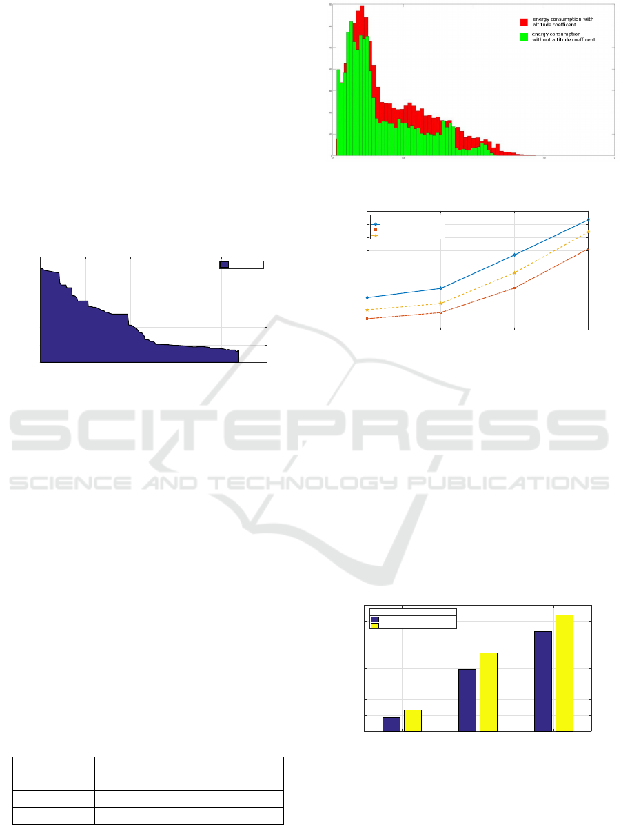
influence the results we report the altimetric path of a
vehicle which is interested to travel through the map
area. This path is reported in Figure 7.
0 500 1000 1500 2000 2500
Traveled Distance [mt]
0
20
40
60
80
100
120
Altitude [mt]
Altimetric Path
Figure 7: Altimetric Path along the map area.
The Probability Density Function (PDF) of the
consumption trend is shown in Figure 8. In this sce-
nario, higher consumptions for the model that con-
sider slope coefficients of roads are measured. The
differences between the consumption of vehicles con-
cerning the altitude coefficient and the driver behav-
ior is presented in Figure 9. In particular, we evalu-
ated the energy consumption of vehicles by changing
the considered map area. Each map presents a differ-
ent average slope coefficient which are summarized
in table 5. Moreover, we evaluate the consumption by
considering different driver style as shown in table 3.
Thus, each point of the line represents results about
average consumption per Km of vehicle with a spe-
cific altitude coefficient and a driver behavior. As ex-
pected when the altitude coefficient of the map raises
also the average vehicle consumption increases. The
same happens regarding the driver behavior: grad-
ually the more the behavior becomes aggressive the
more consumption raises.
Table 5: Slope Coefficients.
Map Name Avg. Slope Coeff. Area Size
Map Area 1 4.50 15.6 Km
2
Map Area 2 3.07 9.5 Km
2
Map Area 3 1.35 10.6 Km
2
The slope coefficient is also important to evalu-
ate energy consumption of vehicles during their travel
Figure 8: Comparison of PDF trend considering map area
with altitude coefficient and not.
Below Normal Normal Aggressive Very Aggressive
0.1
0.15
0.2
0.25
0.3
0.35
0.4
0.45
0.5
Vehicle Consumption vs. Slope coefficient
Higher Altitude Coefficient (4.50)
Lower Altitude Coefficient (1.35)
Medium Altitude Coefficient (3.07)
Legend
Figure 9: Average Energy consumption per Km of vehicles
versus drivers’ behaviors.
along roads. For this reason we perform a dedicated
simulation campaign to evaluate the impact of slope
coefficient for different vehicle class. The vehicle dif-
ferentiate between them because of mass. Considered
vehicles are reported in Table 6. In Figure 10 the
trend of Energy consumption versus vehicle class is
reported. Here it is possible to note how the slope
coefficient influences the overall performances of the
EVs. Moreover, it is possible to note how the mass
of vehicle is related to the overall consumption. This
demonstrates the importance of the slope coefficient
that must be considered in the simulation environment
to achieve a more realistic scenarios.
Renault Twizy ( 460 Kg ) Mitsubishi i-MiEV(1110 Kg) Nissan Leaf (1474 Kg)
Car Type
0
0.1
0.2
0.3
0.4
0.5
0.6
0.7
0.8
Energy Consuption [kW/Km]
Energy Consumption without Altitude
Energy Consumption with Altitude
Legend
Figure 10: Average Energy consumption related to vehicle
class.
SIMULTECH 2018 - 8th International Conference on Simulation and Modeling Methodologies, Technologies and Applications
204

Table 6: Table of vehicles.
Model Brand Mass CdA Efficiency
Twizy Renault 460 0.40 0.8
i-MiEV Mitsubishi 1110 0.75 0.8
Leaf Nissan 1474 0.57 0.8
5 CONCLUSIONS
In this work we propose a new simulation framework
in which simulation environment is much closer to the
real world conditions. Here in the simulation sce-
nario it is possible to consider the altitude and re-
lated roads’ slope coefficient as well as classic pa-
rameters in the modeling of the EVs. Moreover, it
has been proved that the altitude heavily influences
the results and in particular the Energy Consumption
model. Therefore, for considering EV simulation en-
vironment and to evaluate overall behavior it is im-
portant to include the road slope coefficient during the
EV journey. In order to achieve more detailed simu-
lation results, in this work we propose a driver clas-
sification by introducing four driver classes. In fact,
drivers may influences performances in terms of trav-
eling time, road congestion and collisions because of
their behaviors. Moreover, in this work the model was
extending to classic vehicles for better monitoring en-
ergy consumption and emissions. In this way will be
possible to extend this work to design and the develop
of Intelligent Transportation System (ITS) policies in
a further work.
REFERENCES
(2018). Google maps api.
(2018). Open street map.
Bedogni, L., Bononi, L., D’Elia, A., Felice, M. D., Nicola,
M. D., and Cinotti, T. S. (2014). Driving without anx-
iety: A route planner service with range prediction for
the electric vehicles. In 2014 International Confer-
ence on Connected Vehicles and Expo (ICCVE), pages
199–206.
Bieker, L., Krajzewicz, D., Morra, A., Michelacci, C., and
Cartolano, F. (2015). Traffic simulation for all: A real
world traffic scenario from the city of bologna. In
Behrisch, M. and Weber, M., editors, Modeling Mo-
bility with Open Data, pages 47–60, Cham. Springer
International Publishing.
Fazio, P., De Rango, F., and Sottile, C. (2012). An on de-
mand interference aware routing protocol for vanets.
7.
Fazio, P., De Rango, F., Tropea, M., and Voznak, M. (2017).
Cell permanence time and mobility analysis in infras-
tructure networks: Analytical/statistical approaches
and their applications. Computers and Electrical En-
gineering, 64:506–523.
Fazio, P., Rango, F. D., and Sottile, C. (2011). A new in-
terference aware on demand routing protocol for ve-
hicular networks. In 2011 International Symposium
on Performance Evaluation of Computer Telecommu-
nication Systems, pages 98–103.
Gipps, P. (1981). A behavioural car-following model for
computer simulation. Transportation Research Part
B: Methodological, 15(2):105 – 111.
Hemmerle, P., Koller, M., Rehborn, H., Kerner, B. S., and
Schreckenberg, M. (2016). Fuel consumption in em-
pirical synchronised flow in urban traffic. IET Intelli-
gent Transport Systems, 10(2):122–129.
Knospe, W., Santen, L., Schadschneider, A., and Schreck-
enberg, M. (2000). Towards a realistic microscopic
description of highway traffic. Journal of Physics A:
Mathematical and General, 33(48):L477.
Krajzewicz, D., Erdmann, J., Behrisch, M., and Bieker-
Walz, L. (2012). Recent development and applications
of sumo - simulation of urban mobility.
Kurmis, M., Andziulis, A., Dzemydiene, D., Jakovlev, S.,
Voznak, M., and Gricius, G. (2015). Cooperative con-
text data acquisition and dissemination for situation
identification in vehicular communication networks.
Wireless Personal Communications, 85(1):49–62.
Kurmis, M., Voznak, M., Kucinskas, G., Drungilas, D.,
Lukosius, Z., Jakovlev, S., and Andziulis, A. (2017).
Development of method for service support manage-
ment in vehicular communication networks. 15, book-
title =.
Maia, R., Silva, M., Arajo, R., and Nunes, U. (2011). Elec-
tric vehicle simulator for energy consumption studies
in electric mobility systems. In 2011 IEEE Forum on
Integrated and Sustainable Transportation Systems,
pages 227–232.
Olascuaga, L. M. H., Garcia, J. A. R., and Pinzon, J. E. P.
(2015). Evs mass adoption in colombia ; a first ap-
proach model. In 2015 IEEE 15th International Con-
ference on Environment and Electrical Engineering
(EEEIC), pages 1285–1290.
Packer, N. (2011). A beginner s guide to energy and power.
Waraich, R. A., Charypar, D., Balmer, M., and Axhausen,
K. W. (2015). Performance Improvements for Large-
Scale Traffic Simulation in MATSim, pages 211–233.
Springer International Publishing, Cham.
Zhou, X., Tanvir, S., Lei, H., Taylor, J., Liu, B., Rouphail,
N. M., and Frey, H. C. (2015). Integrating a simplified
emission estimation model and mesoscopic dynamic
traffic simulator to efficiently evaluate emission im-
pacts of traffic management strategies. Transportation
Research Part D: Transport and Environment, 37:123
– 136.
A Vehicular Traffic Simulator Model for Evaluating Electrical Vehicle Performances in a Configurable Mobility Scenario
205