O Isotope Concentration Control

Valentin Sita

, Vlad Mureşan

, Mihail Abrudean

, Mihaela-Ligia Ungureşan

and Iulia Clitan

Automation Department, Technical University of Cluj-Napoca, Memorandumului street, no. 28, Cluj-Napoca, Romania

Department of Physics and Chemistry, Technical University of Cluj-Napoca, Memorandumului street, no. 28,

Cluj-Napoca, Romania

Keywords:

O Isotope, Concentration Control, Mathematical Model, Neural Network, Distributed Parameter Process,

Nonlinear System, Independent Variable.

Abstract: The paper presents a solution to control the

O isotope concentration at the output of a separation column.

The proposed mathematical model which describes the work of the separation column is a distributed

parameter one and it approximates with high accuracy the work of the real plant. The isotope separation

process is included in a complex control structure which generates high control performances. In order to

improve significantly the separation column productivity, an original solution for the efficient rejection of

the disturbances effects, is proposed. Also, a solution to determine the instantaneous value of the separation

column length constant is proposed, solution which opens the possibility to implement new control

strategies.

1 INTRODUCTION

The separation column for the

O isotope and the

equipment of the refluxing system necessary for its

work is presented in Fig. 1. In this context, the

isotope separation is made through isotopic

exchange in the system NO, NO

-H

O, HNO

(Abrudean, 1981). In Fig. 1, FSC is the Final

Separation Column, the term “Final” being used due

to the fact that this column works as the final

column of a separation cascade which contains two

separation columns. The main aim of this paper is to

control the FSC work in the case when it works

independently from the separation cascade. The

results of this research activity, consisting from the

proposed control strategy, will be further used in

order to find an appropriate method to control the

separation cascade work.

As it can be remarked in Fig. 1, FSC has the

height h = 10 m, being built from 5 sectors

(S1 – S5), each having the height h/5 = 2 m. The

column diameter is d = 14 mm. The separation of the

O isotope is based on the circulation in FSC, in

counter-current, of the nitric oxides (NO, NO

)

introduced in the lower part of the column and of the

nitric acid (HNO

) – solution introduced in the upper

part of the column. The input flow of nitric oxides is

notated with F

and the output flow of nitric acid is

notated to F

, representing the isotopic waste of the

separation process. F

represents the output flow of

the nitric oxides from FSC which is circulated to the

arc-cracking reactor ACR. At the ACR output, the

flow F

of both nitrogen (N

) and nitric oxides (NO,

) results, with an increased concentration of

. In the absorber A, the absorption of the nitric

oxides in water is made, resulting nitric acid solution

which supplies FSC (the flow of nitric acid solution

is notated with F

). The absorber A is supplied with

the water flow F

H2O

. The amount of nitrogen and

nitric oxide from the absorber output, under the flow

(NO, N

) is sent to the catalytic reactor CR. In

CR, the water with which the absorber is supplied

results through the reaction of nitric oxide (NO) with

hydrogen (H

) (CR is supplied with the hydrogen

flow F

). Also, after the reaction from CR, the

excess of nitrogen and hydrogen results (the flow

The product can be extracted from the top of

FSC under the form of nitric acid with an increase

concentration of

O isotope (HN

). The product

flow is notated with F

and the corresponding pipe is

figured with dashed line due to the fact that in this

paper, only the total reflux (F

= 0) working regime

is approached. The hachure used in Fig. 1 signifies

Sita, V., Mure¸san, V., Abrudean, M., Ungure¸san, M-L. and Clitan, I.

O Isotope Concentration Control.

DOI: 10.5220/0006877403690379

In Proceedings of the 15th International Conference on Informatics in Control, Automation and Robotics (ICINCO 2018) - Volume 1, pages 369-379

ISBN: 978-989-758-321-6

369

the fact that the corresponding elements contain

packing (steel packing in the case of FSC and in the

case of the reactors) and ceramic packing (Axente,

1984) in the case of the absorber. In order to

measure the concentration of the

O isotope, at the

separation column output, a mass spectrometer is

used.

Figure 1: The separation column for the

O isotope and

the equipment of the refluxing system.

2 ISOTOPE SEPARATION

PROCESS MODELLING

The

O isotope separation process is a distributed

parameter one (Colosi, 2013; Li, 2011) due to the

fact that during the separation exchange, the main

output signal (the

O isotope concentration)

depends on two independent variables: time (t) and

the position in FSC length (s). In order to highlight

the position in FSC length, the (0s) axis is defined

(in Fig. 1). The origin (0) of the (0s) axis represents

the centre of the Column Base Section (CBS). The

independent variable (s) has an increasing evolution

from the column base to the column top and its

maximum value can be obtained for s = h,

corresponding to the Column Top Section (CTS).

The main input signal in the process is considered

the input flow of nitric oxides F

(t) and, as it was

previously mentioned, the main output signal from

the process is considered the

O isotope

concentration notated with y(t,s). The mathematical

modelling is made in the hypothesis when FSC

works in total reflux regime (F

= 0). This regime is

used in the first part of the plant working with the

purpose of increasing the

O isotope concentration

until the imposed value, at the column top, is

reached. This working regime is the most relevant

one for the FSC dynamics.

The mathematical model which describes with

high accuracy the work of FSC is proposed in

(Mureşan, 2018). This model is briefly presented in

the following equations. The final form of the output

signal is given by:

s1 0

0f 0f

s1 f 0

F(s) y

y(t,s) y y (t) y y (t)

F(s s h) y

−

=+ ⋅ =+ ⋅

==−

−

(1)

where y

= 0.204% represents the natural abundance

of the

O isotope. Also, the y

(t) function models

the separation process dynamics in relation to time

(t), representing the solution of the ordinary

differential equation:

dy (t)

y(t) u

dt T(F ) T(F )

=− ⋅ + ⋅

(2)

where T(F

) is the isotope exchange process time

constant which depends on the input flow F

(t) and

(t) represents the increase of the

O concentration

over the y

value, in steady state regime. The

previously presented differential equation is solved

considering the remark that firstly the value of the

time constant is singularized for a certain (F

). The

linear variation of the time constant in relation to the

input signal (T(F

)) is given by:

i2Ti2

T(F ) T K (F F )=+ ⋅− (3)

where F

= 185 l/h (implying the time constant

= 84.703 h experimentally determined) and

K 3.9262

=−

represents the gradient of the

ramp T(F

). The u

(t) signal has the following form:

fff 00i

n(F)

tp i

uy(t,ssh)yy(S(F)1)

y( 1)

===−=⋅−=

=⋅α −

(4)

ICINCO 2018 - 15th International Conference on Informatics in Control, Automation and Robotics

370

where t = t

is the final value for time (corresponding

to the steady state regime) and s = s

is the final

value for the independent variable (s)

(corresponding to the column top). Also,

n(F)

tp i

S(F ) =α represents the separation, being a

function which depends on the input signal. In its

equation, α = 1.018 is the elementary separation

factor of the

O isotope for the isotopic exchange

procedure in the system NO, NO

-H

O, HNO

. Also,

the equation of the number of the theoretical plates

is:

tp i

n(F)

HETP(F )

(5)

where HETP (F

) is the Height of Equivalent

Theoretical Plate. Both n

and HETP are functions

depending of the input signal (F

). The HETP

variation is linear on intervals, but is nonlinear on

the entire domain of F

values. The HETP function is

given by the following system of equations (being

linear on intervals, but is nonlinear on the entire

domain of F

values):

i0H1i0i

i0H2i0i

HETP(F ) HETP K (F F ), if F 140 l / h

HETP(F ) HETP K (F F ),if F 140l / h

=+⋅− ≤





=+⋅− >



(6)

where HETP

= 8.6 cm obtained for the input flow

= 140 l/h, and K

, respectively K

(

cm h

K0.08

⋅

=−

for

F 140 l / h≤ ;

cm h

K 0.0333

⋅

for

F 140 l / h> ) are the

gradients of the two ramps from (6) (experimentally

determined). The HETP (F

) function is graphically

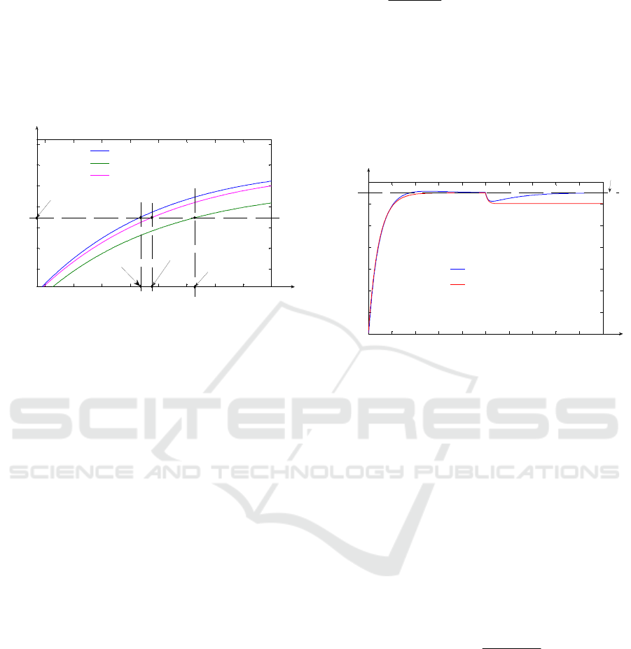
represented in Fig. 2.

Figure 2: The HETP dependency in relation to F

In order to avoid the usage of the two equations

from (6), a neural network is trained to learn the

HETP(F

) function. The structure of the used neural

network is a feed-forward fully connected one

(Haykin, 2009; Vălean, 1996), having one input

signal (F

), one hidden layer (containing 20 neurons)

and one output signal (HETP(F

)). The neurons of

the hidden layer are nonlinear having as activation

function the hyperbolic tangent and the output

neuron is linear. After training, the neural network

output, more exactly the HETP(F

) function, is given

by:

iio

HETP(F ) WL tanh(W F B) b=⋅ ⋅++ (7)

where WL, W, B and b

are the training solutions

(WL is the row vector which contains the input

weights, W is the column vector which contains the

layer weights, B is the column vector which contains

the bias values of the neurons from the hidden layer

and b

is the output neuron bias value). Also, the

notation “tanh” represents the hyperbolic tangent

function.

The

F(s)

−

function from (1) highlights the

proportion of the

O isotope concentration in a

certain position from the FSC height, in relation to

the

O isotope concentration at the FSC top.

Practically, F

(s) function models the concentration

evolution on the column height. The F

(s) function

is obtained using the

s1 0

F(s) y e=⋅ function which

approximates the

O isotope concentration

distribution on the FSC height, for a certain (F

)

(implicitly for a certain HETP(F

)). In the F

(s)

function, (S) represents the “length” constant of the

column and depends on the input signal F

. The S(F

)

function is given by the system of two equations

from (8).

i1S1i1 i

i2S2i2 i

S(F ) S K (F F ), if F 140 l / h

=+ ⋅ − ≤





=+ ⋅− >



(8)

where S

= 751.124 cm obtained for F

= 80 l/h and

= 565.5 cm obtained for F

= 185 l/h. Also, K

and K

(

cm h

K 4.4804

⋅

=−

for

F140l/h≤ ;

cm h

K 1.8489

⋅

for

F 140 l / h> ) are the

gradients of the two ramps from (8) (experimentally

80 100 120 140 160 180 200

8.5

9.5

10.5

11.5

12.5

13.5

Fi [l/h]

HETP [cm]

HETP

O Isotope Concentration Control

371

determined). From (8), it can be remarked that S(F

)

has an evolution linear on intervals, but nonlinear on

the entire domain of F

values. In order to learn the

S(F

) function, the neural structure as in the case of

HETP(F

) function is used, but having 50 neurons in

the hidden layer. After training, the neural network

output, more exactly the S(F

) function, is given by:

iio

S(F ) WL tanh(W F B) b=⋅ ⋅++ (9)

where WL, W, B and b

have the same significance

as in the case of HETP(F

) function. Obviously, WL,

W, B and b

are singularized as values for the S(F

)

function, being the solutions of its corresponding

neural network training.

3 THE PROPOSED CONTROL

STRATEGY

The proposed control structure for the

concentration control is presented in Fig. 3. In

Fig. 3, SDPP represents the Separation Distributed

Parameter Process which has as input signal the flow

of nitric oxides F

(t) and its work depending, also, on

the independent variable (s). The output signal from

SDPP is the

O concentration y(t,s), signal which is

not yet affected by the disturbance effect. The main

disturbance signal modifies directly the value of

SDPP outputs signal, having the value y

(t).

Practically, the final value of the

O concentration

(the final output signal) is y

(t,s) = y(t,s) + y

(t). DD

is the disturbance delay element, modelling the

disturbance propagation into the process and y

the steady state value of the disturbance. The main

disturbance signal in the control system is

represented by the product extraction flow (F

Even, the product extraction is a usefully procedure,

it can be assimilated with a disturbance due to the

fact that extracting (HN

), with an increased

concentration of

O, from the column, the

isotope concentration in the column decreases. The

concentration of

O isotope is measured using the

concentration sensor CS which is a mass

spectrometer and generates the feedback signal r

(t).

The automation equipment (Golnaraghi, 2009; Love,

2007) from the

O isotope control system works

with unified current signals (4 – 20 mA), obviously

(t) being an unified current signal. The actuating

signal (F

(t)) is generated by the actuator, in this case

the nitric oxides pump P. MSFP represents the

reference Model of the System Fixed Part (which

includes the mathematical models of the pump P, of

SDPP and of the sensor CS, serial connected). It is

run on a process computer in parallel with the real

process, having its initial (reference) behaviour (not

affected by the exogenous disturbances (y

(t) = 0)

and not affected by parametric disturbances). The

SDPP is integrated in MSFP by implementing the

mathematical model presented in Section 2. Also,

the mathematical models of P and CS are integrated

in MSFP by implementing for each a neural

network. The two neural networks have nonlinear

autoregressive structure with exogenous inputs

(NARX), they contain, each, 9 linear neurons in the

hidden layer (they have only one hidden layer) and

one linear neuron in the output layer, respectively

they have, each,

two unit delays (one on the input

signal and one on the output signal, due to the fact

that P and CS are first order systems).

The main error signal is e

(t) = w(t) – r

(t), where

w(t) is the concentration setpoint signal. The main

concentration controller CC of PID (Proportional –

– Integral – Derivative) type, processes the signal

(t) and generates the main control signal c

(t). The

secondary error signal e

(t) = r

(t) – r

(t), where r

(t)

is the feedback signal generated at the output of

MSFP, represents the measure of the effects of all

disturbances (both exogenous and of parametric

type) which occur in the system. Practically, e

(t) is

a measure of the deviation of the output signal value

in relation to its reference value (generated by the

simulation of MSFP). For a correct comparison

between the real plant behaviour (referring to the

fixed part) and its reference model behaviour, at the

input of both entities, the same input signal c

(t) is

applied. The mentioned parametric disturbances can

be of two types: the small variations in relation to

time of the separation column structure parameters

or the small variations of (s) independent variable

(due to the change of the CS position and of the

product extraction point; due to this aspect, the

reference model is simulated for s = s

). The

disturbances compensator DC of PD type

(Proportional – Derivative) processes the error

signal e

(t) and generates the compensation control

signal c

(t). The total control signal due to the

control efforts of CC and DC results as

(t) = c

(t) – c

(t). The final control signal c

(t)

results as c

(t) = c

– c

(t), where c

represents the

value, in unified current, proportional with the value

of the reference flow. The reference flow is referring

to the initial flow at which the separation column

starts to work.

From (3), the fact the lowest value of the

separation column time constant is obtained for the

flow F

ICINCO 2018 - 15th International Conference on Informatics in Control, Automation and Robotics

372

Figure 3: The proposed control structure.

Consequently, in order to obtain an acceptable

value of the concentration control system settling

time, the reference flow is fixed at the value of F

Also, other values could be chosen for the reference

flow (for example F

) but we would obtain a slower

control system. The element IF (Initial Flow)

generates the value F

which is scaled to the c

value

using the proportionality constant K1.

The instantaneous value of (s) independent

variable is determined using LIVIE (Length

Independent Variable Identification Element), more

exactly the sensor position in the column. This

procedure is necessary in order to determine if the

separation plant can be physically used when the

sensor position in the column is changed. Another

advantage of this procedure is the possibility to

equivalate the disturbances effects with the change

of the CS position in the column. The work of

LIVIE is based on obtaining the F

(s) function from

the ratio between the feedback signals r

(t) and

(t), resulting the signal a(t) (

r(t)

a(t)

r(t)

). The

feedback signals r

(t) and r

(t) result as differences

between the primary feedback signals r

(t),

respectively r

(t) and r

, which is the value in unified

signal corresponding to the

O natural abundance

). The value of (y

) is generated by NA (Natural

Abundance Element), after that it being scaled with

the proportionality constant K2, resulting (r

Obviously, at the plant work starting, r

(t) is

initialized at a value different than 0, in order to

make possible the computation of a(t). The

instantaneous value of the independent variable (s),

notated with (s

), can be obtained from the equation

of F

(s), being given by:

S(F (t ))

s S(F (t)) ln[a(t) e (1 a)]=⋅⋅+−

(10)

The numerical implementation of (10) is made

by LIVIE. The two input signals in LIVIE are a(t)

and F

(t) which is the approximated value of the

actuating signal F

(t). The signal F

(t) is generated

by the simulation of PM (Pump Model) element,

which is implemented using the same procedure as

in the case of MSFP and having as input signal the

(t) signal. The natural logarithm and the

exponential function from (10) are numerically

implemented using feed-forward fully connected

neural networks, too. The Decision Element (DE)

generates the “DECISION” in relation to the

identified value of (s

). The “DECISION” can be the

generation of an alarm if the (s

) variable tends to

reach the limit value or the separation plant stop if

) variable equals the imposed limit.

In case of the real separation plant, the following

elements from Fig. 3: CC, DC, MSFP, LIVIE, PM,

IF, K1, NA and K2 have to be implemented on

numerical equipment. In order not to increase Fig. 3

complexity in a non-understandable manner, the

analog to digital and the digital to analog converters

O Isotope Concentration Control

373

which connect the numerical equipment to the

separation plant are not figured.

4 CONTROLLERS TUNING AND

SIMULATIONS RESULTS

The simulations presented in this paper are made in

MATLAB/Simulink. The CC tuning is made not

considering the disturbances action in the system

= 0 and s = s

) and, also, not considering the DC

control action (c

(t) = 0). Due to the fact that the

isotope separation process, besides being a

distributed parameter process, is a strong nonlinear

one, the relay method is used for CC tuning. In order

to obtain an oscillatory variation of the output signal

y(t,s), the CC controller is replaced with a two

position relay having the output commutation

between the value b

min

= 0 mA and the value

max

= 6.4 mA (without considering the initial value

of 4 mA for the unified current signals), respectively

having the hysteresis set to ±1 mA.

If the simulation is made for a step type setpoint

signal (proportional with the imposed value of 1.5 %

for the output

O isotope concentration), the control

system response (the variation in relation to time of

the y(t,s) signal) is presented in Fig. 4.

Figure 4: The control system response in the case of the

relay tuning method application.

In Fig. 4, the fact that the constant amplitude

oscillations are obtained, after 1000 h from the

simulation start, is highlighted. From Fig. 4, the

oscillation period T

OSC

= 552 h and the oscillation

amplitude A

OSC

= A/2 = 0.0907 % result. Using the

values obtained for T

OSC

and A

OSC

, the parameters of

the PID CC controller can be computed using the

Ziegler – Nichols equations. The PID controller

transfer function is:

DCC

CC CC

ICC fCC

H(s)K (1 )

TsTs1

⋅

=⋅+ +

⋅⋅+

(11)

where K

is the controller proportionality constant,

ICC

is the controller integral time constant, T

DCC

the controller derivative time constant and T

fCC

is the

time constant of the first order filter used to make

the PID controller feasible. After the application of

Ziegler – Nichols equations, the fine tuning of the

controller is made in order to obtain better control

performances. The fine tuning consists in modifying

the initial form of the obtained controller parameters

and in testing the control performances variation,

until the best set of performances is obtained. At the

tuning procedure end, the following parameters are

obtained: K

= 0.358, T

ICC

= 197.143 h,

DCC

= 33.12 h and T

fCC

= 0.625 h. If the setpoint

concentration is set to 1.5%, the comparative graph

between the separation process open loop response

and the control system responses for the cases of

using the best PI controller that could be obtained

respectively using the proposed PID controller, is

presented in Fig. 5. In Fig. 5, the notation CSt

signifies the minimum concentration value of the

steady state band near the steady state value of the

output signal (the steady state band is fixed at ±2%,

more exactly CSt = 1.47 %).

Figure 5: The comparative graph between the open loop

separation process response and the control system

responses using two different controllers.

From Fig. 5, it results that in all three simulation

cases, the steady state error e

= 0 %, due to the fact

that, in steady state regime the three curves reach the

imposed value for

O concentration (y

= 1.5 %).

Also, in the case of using both controllers, a small

overshoot occurs, having the value smaller than 1 %

(the maximum imposed limit). The PID controller

generates the overshoot σ

= 0.94 %, insignificantly

higher than σ

= 0.9 % (generated by the

PI controller). Obviously in the case of the

separation process open loop response the overshoot

0 500 1000 1500 2000 2500 3000 3500 4000 4500 5000

0.2

0.4

0.6

0.8

1.2

1.4

1.6

1.8

TIME [h]

O CONCENTRATION [%]

TOSC

0 500 1000 1500 2000 2500

0.2

0.4

0.6

0.8

1.2

1.4

1.6

TIME [h]

O CONCENTRATION [%]

Case of PID Controller

Open loop response

Case of PI controller

ts1

CSt

ICINCO 2018 - 15th International Conference on Informatics in Control, Automation and Robotics

374

is σ

= 0 %. Due to the fact that in all three cases the

overshoot is included in the steady state band, the

settling time (which is a critical performance) is

considered when the curves from Fig. 5 reach the

CSt value. In Fig. 5, the fact that the PID controller

generates the smallest settling time t

, results. In

order to distinguish the three values of the settling

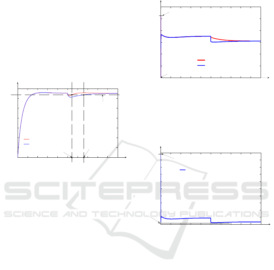
times, Fig. 6 is considered.

Figure 6: The settling times associated to the three curves

from Fig. 5.

From Fig. 6, the fact that the PID controller

generates the best settling time (t

= 719.58 h) is

highlighted. It can be remarked that t

< t

= 740.21 h and t

= 819.92 h). Consequently, the

PID controller usage, improves significantly the

separation plant settling time implying important

economic advantages. Also, using the PID

controller, even better settling times were obtained

in simulations, but only if the actuating signal exits

from allowed variations limits. Practically, t

represents the best settling time that could be

obtained if the actuating signal (F

(t)) remains

enclosed between the saturation limits. The open

loop separation process simulation is made

simulating the mathematical model presented in

Section II for the input flow F

= 150.255 l/h, value

which generates the steady state value of 1.5 % for

the output

O concentration (according to (3) and

(6), the best settling time for the open loop process,

if we impose a certain value of the output signal, is

obtained if F

(t) > 140 l/h). The main problem in the

case of usage the separation process in open loop is

the fact that the effect of the disturbances cannot be

rejected, aspect highlighted in Fig. 7. The

simulations from Fig. 7 are made in the same

conditions as the simulations from Fig. 5, but the

exogenous disturbance with the value y

= − 0.1 %

occurs in the system at the moment t

= 2500 h.

The y

value is propagated in the system through

the DD element having the transfer function

H(s)

Ts1

⋅+

, where the time constant

= 50 h. Also, the negative value of y

physically interpreted as the output

O isotope

concentration decrease, due to the exogenous

disturbance effect. From Fig. 7, it results that in the

case of the PID controller usage, the disturbance

effect is rejected, in steady state regime the system

response reaching again the imposed value

= 1.5 %).

Figure 7: The exogenous disturbance effect.

The open loop response of the separation

process, after the disturbance occurs in the system,

gets steady to the value y

st1

= 1.4 % (with y

smaller

than y

, resulting that the disturbance effect is not

rejected) fact which highlights again the necessity of

using a controller for the concentration control. An

important problem which results from Fig. 7 is the

slow reaction of the control system in disturbance

rejecting regime (the duration of the transitory

regime implied by the disturbance effect is over

800 h). In this context, the necessity of using the DC

element occurs. For the structure of the Disturbance

Compensator (DC) a PD transfer function is

proposed, it having the form:

DDC

DC DC

fDC

Ts1

H(s)K

Ts1

⋅+

=⋅

⋅+

(12)

The tuning procedure of DC follows the stages:

firstly the proportionality constant of DC is

initialized at the value K

= 1, its derivative time

constant is initialized at the value T

DDC

= 10 h,

respectively the time constant of the first order filter

used to obtain the feasible form of DC is fixed at the

value T

fDC

= 1 h; secondly, T

DDC

is iteratively

determined by increasing its value from an iteration

to the next one with ∆T

DDC

= 1 h until the system

response overshoot in disturbance effect rejecting

regime occurs (the overshoot values are determined

550 600 650 700 750 800 850 900

1.42

1.44

1.46

1.48

1.5

1.52

1.54

TIME [h]

O CONCENTRATION [%]

Case of PID Controller

Open loop response

Case of PI controller

ts1

ts3

ts2

CSt

0 500 1000 1500 2000 2500 3000 3500 4000 4500 5000

0.2

0.4

0.6

0.8

1.2

1.4

1.6

O CONCENTRATION [%]

TIME [h]

The case with PID Controller

The open loop response

yst

O Isotope Concentration Control

375

repeating the simulation at each iteration); finally,

is iteratively determined by increasing its value

from an iteration to the next one with ∆K

= 0.01

until the system response overshoot in disturbance

effect rejecting regime equals the system response

overshoot in starting regime (σ

). After the

application of the presented algorithm, the structure

parameters of DC result: K

= 1.1, T

DDC

= 50 h.

The comparative graph between the system response

in the case of using and the case of not using the DC

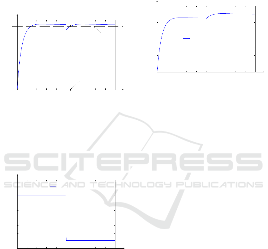
element, is presented in Fig. 8.

Figure 8: The effect of using DC.

The simulations from Fig. 8 are made in the

same conditions as the simulations from Fig. 7.

From Fig. 8, it results that the control system

generates much better performances in disturbance

rejecting regime in the case of using DC than in the

case without DC. Relative to the moment t

(when

the disturbance signal occurs in the system), in the

case of using DC, the

O concentration reaches

again the steady state regime after 219.4 h

(corresponding to the moment t

). This transitory

regime is much shorter than in the context of not

using DC (in this case the

O concentration reaches

again the steady state regime after 842.7 h

(corresponding to the moment t

)). Consequently,

the usage of DC implies a consistent improvement

of the system performances in rejecting the

disturbances effects, fact which represents a major

technological and economical advantage. The

control effort is highlighted in Fig. 9.

From Fig. 9, it results that the variation of the

input flow of nitric oxides is enclosed only between

the saturation limits [F

], aspect which proves that

the usage of the two controllers (CC and DC) is

feasible. Also, in disturbance effect rejecting regime,

due to the action of DC, the actuating signal has a

much faster variation, fact which signifies a much

stronger control effect and implicitly a higher

efficiency of the control system.

Figure 9: The variation, in relation to time, of the actuating

signal.

In Fig. 10, the evolution in relation to time of

HETP(F

) function is presented. This evolution is

associated to the system response presented in

Fig. 8, in the case of using DC.

Figure 10: The variation in relation to time of HETP(F

)

function.

From Fig. 10, it results that the limit values of

HETP(F

) presented in Fig.2 (HETP

min

= 8.6 cm) and

(HETP

max

= 13.4 cm) are almost reached (but not

equalled) only in transitory regimes due to the CC,

respectively DC actions. This aspect proves again

the physical possibility to implement the proposed

control strategy. In Fig. 11, the control system

response is presented in the case of the (s)

independent variable variation. The variation occurs

at the moment t

= 2500 h from the simulation start,

when (s) independent variable value is changed from

the initial value s = s

= 1000 cm) to the value

s = 970 cm. This variation is due to the

concentration sensor position change in relation to

the column height. In Fig. 11, the fact that the two

control elements (CC and DC) reject the effect of the

(s) independent variable value “jump”, is

0 500 1000 1500 2000 2500 3000 3500 4000 4500 5000

0.2

0.4

0.6

0.8

1.2

1.4

1.6

TIME [h]

O CONCENTRATION [%]

The case with DC

The case without DC

ts4

ts5

Cst

0 500 1000 1500 2000 2500 3000 3500 4000 4500 5000

100

120

140

160

180

200

TIME [h]

NIT RIC O X IDES IN PU T F LO W [l/h]

The case without DC

The case with DC

0 500 1000 1500 2000 2500 3000 3500 4000 4500 5000

8.5

9.5

10.5

11.5

12.5

13.5

TIME [h]

HETP [cm]

HETP(Fi) function in relation to time

HETPmax

HETPmin

ICINCO 2018 - 15th International Conference on Informatics in Control, Automation and Robotics

376

highlighted. Only after 237.8 h (corresponding to the

moment t

) from the moment t

, the

concentration equals the CSt value, the imposed

steady state regime (near the value y

= 1.5 %) being

reached again.

Figure 11: The system response, in the case of the (s)

independent variable variation.

This aspect proves the fact that the proposed

control structure can efficiently manage the effect of

the parametric disturbances, too. The (s)

independent variable value change is identified by

the LIVIE element. The variation in relation to time

of the LIVIE output signal (the approximation (s

) of

the (s) instantaneous value) is presented in Fig. 12.

Figure 12: The variation in relation to time of the (s

)

signal.

It can be remarked the fact that the

approximation of the (s) independent variable is an

exact one both before and after the variation moment

In the case when the position of the

concentration sensor remains in the position given

by s = 970 cm, the

O isotope concentration

evolution, in relation to time, for the value s = s

, is

presented in Fig. 13. From Fig. 13, it results that the

O isotope concentration increases at the column

top (s = s

). This aspect is explained through the

increasing evolution of the output signal in relation

to (s) independent variable (according to (1)).

Figure 13: The output signal evolution, in relation to time,

for s = s

The change of the concentration sensor position

has an important application, more exactly when,

immediately after the extraction of the necessary

isotope quantity at the imposed concentration (in the

example 1.5 %), the isotope extraction at a higher

concentration is necessary (for example 1.6 %). In

this case, firstly the extraction is made from the

point s = 970 cm, where the control is made and

secondly, when the

O isotope concentration has to

be increased, the extraction point is changed to

s = s

= 1000 cm (the sensor position can be, also,

changed to the column top). The main advantage

consists in the avoidance of a new transitory regime

and implicitly in a much faster extraction of the

isotope at an increased concentration. The procedure

of identifying the (s) independent variable value can

be, also, used in order to determine if the separation

plant can be physically used. The constrain

regarding the possibility of usage the separation

plant consists in limiting the maximum deviation of

the (s) independent variable with more than 40 cm in

relation to (s

) value. In this context, the equivalent

value of (s) has to be approximated (containing the

superposition of the physical value of (s) and also

the equivalent value of (s) (which represents a

measure of the exogenous disturbances equated as a

position variation in the column height)). In Fig. 14,

the same simulation as in the case of Fig. 11 is

presented (on the first 5000 h), but considering the

fact that at the moment t

= 5000 h, an exogenous

disturbance with the value y

= − 0.2 % occurs in

the system.

In Fig. 14, the moment t

is highlighted with the

ellipse 1 and the moment t

is highlighted with the

ellipse 2. In both cases, the effect of the disturbance

0 500 1000 1500 2000 2500 3000 3500 4000 4500 5000

0.2

0.4

0.6

0.8

1.2

1.4

1.6

TIME [h]

O CONCENTRATION [%]

O Isotope Concentration

ts6

CSt

0 500 1000 1500 2000 2500 3000 3500 4000 4500 5000

965

970

975

980

985

990

995

1000

1005

1010

TIME [h]

s1 [cm ]

s1 Independent Variable [cm]

0 500 1000 1500 2000 2500 3000 3500 4000 4500 5000

0.2

0.4

0.6

0.8

1.2

1.4

1.6

1.8

TIME [h]

O CONCENTRATION [%]

O Concentration for s = sf

O Isotope Concentration Control

377

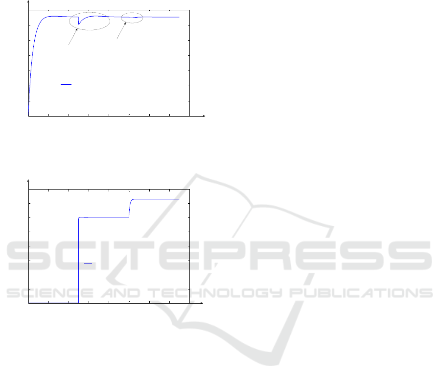
is rejected efficiently, the output signal having in all

steady states the imposed value (1.5 %). The

evolution, in relation to time, of the signal resulted

as the difference (s

– s

), is presented in Fig. 15.

Figure 14: The output signal evolution in relation to time,

when both parametric and exogenous disturbances occur

in the system.

Figure 15: The evolution of (s) independent variable in

relation to (s

Practically, the representation from Fig. 15

signifies the equivalent position of the concentration

sensor in relation to the column top. After the

moment t

, the value of the signal from Fig. 15

increases with 7 cm (due to the exogenous

disturbances). Due to the fact that the maximum

value of the signal from Fig. 15 is 37 cm (value

smaller than the maximum imposed limit – 40 cm),

the conclusion that the system is physically usable at

the considered disturbances values, results. At the

limit of 40 cm, the effect of the disturbances cannot

be rejected without the increase of the actuating

signal over the saturation limits. At the detection of

the value (s

– s = 37 cm) the DE element from

Fig. 3 takes the DECISION of emitting an Alarm

and at the detection of the limit value

– s = 40 cm), the DE element takes the

DECISION of stopping the separation plant.

Obviously, the difference (s

– s) is always positive

due to the fact that the sensor position can be

changed only in the column volume (and only near

its top).

5 CONCLUSIONS

In this paper, an original control structure used for

the control of the

O isotope concentration (isotope

produced using a separation column), is presented.

An important achievement is represented by the fact

that the separation process, which is a distributed

parameter process, is included in a control system.

In order to obtain high control performances in

disturbance rejecting regime, a compensation loop,

based on the process reference model, is designed.

The HETP variation in relation to F

is nonlinear

due to the following explanations: at the consistent

decrease of F

, the steel packing of FSC is not

properly wet and the contact between the liquid and

the gas from the column is not an efficient one, fact

which implies a high value of HETP; at the

consistent increase of F

, the formation of the

flooding phenomenon occurs, fact which implies a

high value of HETP, too; the column optimum

HETP (the smallest value of HETP) is obtained in

the case of the studied separation column for

= 140 l/h which is an intermediary value; each

separation column has an optimum point given by its

optimum loading.

Considering the previous remarks regarding the

HETP value variation, the saturation limits of the

actuating signal are determined, obtaining the

, F

] domain.

Another original element proposed in the paper

is the design of an identification system of the exact

concentration sensor position in the neighbourhood

of the column top. Also, a procedure to equivalate

the disturbances effects, with a change of (s)

independent variable value, is proposed. These

mathematical mechanisms can be used in order to

optimize the product extraction from the separation

plant, when the future orders (for

O isotope) can be

predicted.

Another application of these mathematical

mechanisms is represented by the possibility to

determine if the separation plant is physically usable

and in the case when it is not, the decision element

can take the decision of stopping the plant work.

A future possibility to improve the control

system performances is given by the possibility to

replace the main CC PID controller with an

advanced controller (Kern, 2015; Zou, 2017). Also,

0 1000 2000 3000 4000 5000 6000 7000 8000

0.2

0.4

0.6

0.8

1.2

1.4

1.6

TIME [h]

O CONCENTRATION [%]

O Isotope Concentration

0 1000 2000 3000 4000 5000 6000 7000 8000

TIME [h]

s VARIATION IN RELATION TO sf [cm]

s Independent Variable in Relation to sf

ICINCO 2018 - 15th International Conference on Informatics in Control, Automation and Robotics

378

the proposed model can be extended in order to

obtain the mathematical model of a separation

cascade, which contains two separation columns in

its structure. Obviously, for the case of a separation

cascade, the proposed control strategy has to be

adapted.

REFERENCES

Abrudean, M., 1981. Ph.D. Thesis.

Axente, D., Abrudean, M., Bâldea, A., 1994.

C Isotopes Separation trough Isotopic

Exchange, Science Book House.

Coloşi, T., Abrudean, M., Ungureşan, M.-L., Mureşan, V.,

2013. Numerical Simulation of Distributed Parameter

Processes, Springer.

Golnaraghi, F., Kuo, B. C., 2009. Automatic Control

Systems, 9

edition, Wiley Publishing House.

Haykin, S., 2009. Neural Networks and Learning

Machines, Third Edition, Pearson Int. Edition.

Kern, R., Shastri, Y., 2015. Advanced control with

parameter estimation of batch transesterification

reactor, In Journal of Process Control, Vol. 33, pp.

127-139.

Li, H.-X., Qi, C., 2011. Spatio-Temporal Modeling of

Nonlinear Distributed Parameter Systems:

A Time/Space Separation Based Approach, 1st

Edition, Springer.

Love, J., 2007. Process Automation Handbook, 1 edition,

Springer.

Mureşan, V., Abrudean, M., Ungureşan, M.-L. Coloşi, T.,

2018. Modeling and Simulation of the Isotopic

Exchange for 18O Isotope Production, proposed for

publishing to AQTR, Cluj-Napoca, Romania.

Vălean H., 1996. Neural Network for System

Identification and Modelling. In Proc. of Automatic

Control and Testing Conference, Cluj-Napoca,

Romania, 23-24 May, pp. 263-268.

Zou, Z., Wang, Z., Meng, L., Yu, M. Zhao, D., Guo, N.,

2017. Modelling and advanced control of a binary

batch distillation pilot plant, In Chinese Automation

Congress (CAC), 20-22 October.

O Isotope Concentration Control

379