Learning-based Kinematic Calibration using Adjoint Error Model

Nadia Schillreff and Frank Ortmeier

Chair of Software Engineering, Otto-von-Guericke-University Magdeburg, Germany

Keywords:

Modeling, Parameter Identiﬁcation, Product of Exponentials (POE).

Abstract:

A learning-based robot kinematic calibration approach based on the product-of-exponentials (POE) formula

and Adjoint error model is introduced. To ensure high accuracy this approach combines the geometrical and

non-geometrical inﬂuences like for e.g. elastic deformations without explicitly deﬁning all physical processes

that contribute to them using a polynomial regression method. By using the POE formula for kinematic

modeling of the manipulator it is ensured that kinematic parameters vary smoothly and used method is robust

and singularity-free. The introduced error parameters are presented in the form of Adjoint transformations

on nominal joint twists. The calibration process then becomes ﬁnding a set of polynomial functions using

regression methods that are able to reﬂect the actual kinematics of the robot. The proposed method is evaluated

on a dataset obtained using a 7-DOF manipulator (KUKA LBR iiwa 7 R800). The experimental results show

that this approach signiﬁcantly reduces positional errors of the robotic manipulator after calibration.

1 INTRODUCTION

For a robot manipulator that is mainly used in repet-

itive applications (e.g. pick-and-place operations)

where the desired poses (position and orientation) of

the manipulator’s end-effector (EE) can be manually

taught, high repeatability is important to successfully

perform deﬁned tasks. This ability to repeat a known

pose has submilimeter values (e.g. 0.1 mm for KUKA

LBR iiwa 7 R800) for modern manipulators. How-

ever if a task is unique, the robot is mostly given a

target pose deﬁned in some relative or absolute co-

ordinate system. Such situations arise often when

robot’s poses are obtained through a simulation dur-

ing which the layout of the working environment and

a model of the robot are used. This requires special at-

tention to the accuracy of the simulated robot model,

and whether it corresponds to the robots actual kine-

matics.

This process, known as robot calibration, consists

of developing a mathematical model and identiﬁca-

tion of parameters that are able to reﬂect the actual

behavior of the investigated robot and as a result bet-

ter predict its resulting poses can be build. There are

three categories of calibration presented in the liter-

ature (Elatta et al., 2004). The ﬁrst is joint calibra-

tion, which is also called ﬁrst level calibration, where

the difference between the actual joints displacements

and the encoder signals is considered. Level two in-

volves kinematic calibration, where the robots kine-

matic parameters are determined. Level three takes

into account non-kinematic error sources like elastic-

ity of the links or the backlash of the joints.

One of the most important stages of a calibration

procedure is the modeling stage, namely the selection

of an apropriate kinematic model and speciﬁcation

of its parameters for error identiﬁcation. Among the

most widely used methods to model robot kinematics

is the Denavit-Hartenberg approach (Denavit, 1955)

that uses 4 parametrs to describe relations between

frames of the manipulator. However, if the robot has

consecutive revolute joints with near parallel axes it

can lead to convergence problems during parameter

identiﬁcation. Later Hayati and Mirmirani modiﬁed

this approach by ading an extra parameter of rota-

tion about an axis orthogonal to the plain in which

these parallel axes lie(Hayati and Mirmirani, 1985).

Other methods that address this problem include for

e.g. a Zero-Reference model (Mooring, 1983) and

CPC model (Zhuang et al., 1992).

The POE model, which uses twist theory to de-

scribe the geometry of each joint and is also a zero

reference position method, has been widely used in

robotics ﬁeld. Kinematic parameters of the mod-

els based on the POE formula vary smoothly with

changes of joint axes, resulting in a continuous pa-

rameterization and no singularities for any type of

robot. In general methods that use POE models differ

by the type of the error assignment: additive (Chen

et al., 2014) or multiplicative (Li et al., 2016), and

372

Schillreff, N. and Ortmeier, F.

Learning-based Kinematic Calibration using Adjoint Error Model.

DOI: 10.5220/0006870403720379

In Proceedings of the 15th International Conference on Informatics in Control, Automation and Robotics (ICINCO 2018) - Volume 2, pages 372-379

ISBN: 978-989-758-321-6

by the choice of frames where joint twists are related:

global (Okamura and Park, 1996) or local (Chen et al.,

2001).

Non-kinematic errors are often attributed to elastic

deformations, transmission nonlinearities, and ther-

mal expansion. To account for these errors corre-

sponding effects are analytically expressed with gear

or elastic models as in (Klimchik et al., 2015) or

(Marie et al., 2013). However, this approach depends

on having an accurate representation of the different

processes that can potentialy inﬂuence the accuracy of

the manipulator and inclution of additional parametrs

to be identiﬁed (e.g. moments of inertia of the robot

links, friction parameters). As a result these physical

processes are often simpliﬁed, leading to inaccuracies

in the model.

Instead, learning approaches are proposed to

model the behaviour of a robot. This allows us to

solve the calibration problem as a function estima-

tion task based on the measured data. The learning

approach requires no a-priori knowledge of the phys-

ical model. Instead, the model can be obtained di-

rectly using measured data. By not attributing errors

to speciﬁc physical processes we can distribute kine-

maticic and non-kinematic inﬂuences over introduced

error parameters. In general errors of the robot’s EE

may originate from ﬁve factors (Liou et al., 1993):

environmental (e.g. temperature or the warm-up pro-

cess), parametric (e.g. Kinematic parameter varia-

tion due to manufacturing and assembly errors, inﬂu-

ence of dynamic parameters, friction and other non-

linearities), measurement (resolution and nonlinearity

of joint position sensors), computational (computer

round-off and steady-state control errors) and appli-

cation (e.g. installation errors). To be able to reﬂect

different inﬂuences in the model, experiments that in-

clude variations of the relevant factors would have to

be conducted. This work considers the inﬂuence of

only a limited amount of described factors, mainly

concentrating on the internal parameters of the robot.

However due to the nature of the proposed method,

in case the proper experimental data is available the

model could be easily extended to include other pa-

rameters.

In this paper, a learning based method for robot

calibration using Adjoint error model is presented

along with a comparison of different modeling ap-

proaches. The output of the calibration procedure is

a trained model that based on the input variables (e.g.

robot joint values and nominal Cartesian position of

the EE) would calculate the resulting pose of the ma-

nipulator under the inﬂuence of kinematic and non-

kinematic errors. This model can then be applied to

more accurately plan the tasks of the manipulator.

This paper is organised as follows. In Section 2,

the forward kinematics based on POE formula along

with the Adjoint error model are presented. A method

to calculate the values of the introduced error parame-

ters based on measurement data is introduced. We de-

scribe different modeling techniques in Section 3. In

Section 4, the proposed method is applied to the per-

formance evaluation of a KUKA LBR iiwa 7 R800

manipulator and the modeling thechniques are com-

pared. We conclude our paper in Section 5.

2 ROBOT KINEMATIC AND

ERROR MODELING USING

POE FORMULA

In this section, a method applied for calculation of

error parameters is described. First the POE repre-

sentation and Adjoint error model is used to describe

the robotic manipulator. After that the difference be-

tween reference poses of a robots ﬂange measured

by a tracking system and the corresponding nominal

poses of the robot is used to obtain the values of the

introduced error parameters.

2.1 Robot Kinematic Model

According to Brockett (Brockett, 1984), the POE

model needs two coordinate frames attached in an ar-

bitrary position. Typicaly a frame S is attached to the

robot base link and a tool frame T to the EE. The rigid

displacement of T with respect to S can be described

by a 4 × 4 homogeneous matrix g

as:



R p

0 1



(1)

where R

3×3

∈ SO(3) is an orthogonal matrix de-

scribing coordinate axes of T in S and p

3×1

∈ R

the position vector of the origin of T in S.

Each joint of the manipulator is associated with a

twist ξ

, i = 1, . . . , n, of the Lie algebra se(3) of SE(3)



0 0



(2)

where v

= [v

, v

]

∈ R

and

∈ so(3) is a

skew symmetric matrix of w

= [w

, w

]

∈ R

and is given by:





0 −w

−w





(3)

The twist

can also be expresed as a 6×1 vector

= (v

, w

)

∈ R

. For a revolute joint, w

is the

Learning-based Kinematic Calibration using Adjoint Error Model

373

direction unit vector of the joint axis and v

= q

×w

where q

is an arbitrary point on the joint axis. For a

prismatic joint, w

= 0, and v

gives the unit direction

of the joint axis.

Then, the forward kinematic model of a serial

robot maping joint variables Θ

Θ = [θ

, . . . , θ

]

to the

tool frame displacement g

based on the POE for-

mula can be expressed as (Murray et al., 1994):

= e

···e

, (4)

where the matrix exponential e

is the motion

generated by joint i with joint variable θ

, and g

denotes the initial tool frame displacement when all

joint angles are set to zero.

2.2 Adjoint Error Model

Based on the observed discrepancies between the

nominal kinematic model of the robot and measured

data, the current robot model has to be extended with

error parameters, that can reﬂect the differences in the

pose of the EE.

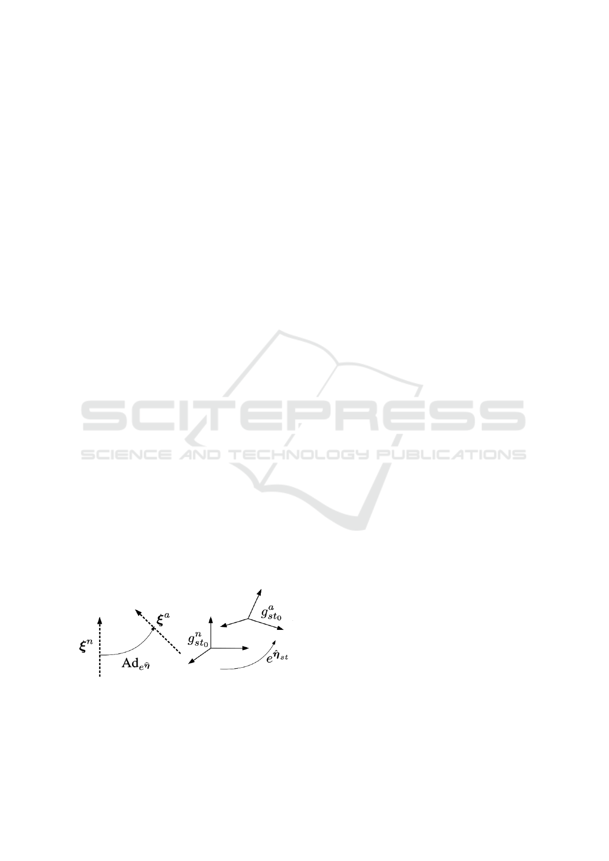
Li et al. proposed a multiplicative Adjoint trans-

formation error of the twist coordinates, referred to

as Adjoint error. According to this model the rela-

tionship between an actual joint twist and a nominal

joint twist, as shown in Figure 1, is given by (Li et al.,

2016):

= Ad

(5)

for error parameters η

η = (v

, w

)

∈ se(3). Ad-

joint transformation of the twist ξ

ξ with g

g = (R

R, p

p) is

given by (Murray et al., 1994):

ξ =



0 R



ξ (6)

And the error of the initial tool frame offset g

can be expressed by:

= e

(7)

Figure 1: Adjoint error model for joint twists and offset of

the tool frame.

2.3 Error Parameters Calculation

After deﬁning an appropriate error model the intro-

duced error parameters should be estimated based on

the experimental data. The measured reference pose

of a point i, g

, can be written in general form as:

= f

H), (8)

where f

is a non-linear function of H

H =

[η

, . . . , η

, η

], a vector containing introduced error

parameters for each joint and initial tool frame offset.

Since these errors are small, this function can be lin-

earized at point H

H = 0

0. This is equivalent to having

all error parameters equal to 0:

= f

0) + J

H|0

H − 0

0), (9)

where J

H|0

is a Jacobian function of f

with re-

spect to the elements of error vector H

H, evaluated at 0

(denoted as J

in the following).

Because f

0) corresponds to the pose calculated

with the nominal parameters g

, given by Equation 4,

the difference between nominal and measured pose,

∆g

, is:

∆g

= J

H (10)

If there are l measurements available, we can

present Equation 10 in matrix form as:

∆g







∆g



















H = J

H (11)

Under assumption that introduced error parame-

ters are constant, the above equation can be solved

with a least squares technique using a left pseudo-

inverse matrix of J

. But considering the need to

include the non-geometric inﬂuences (which are con-

ﬁguration dependent and as result can not be constant)

into developed model, this approach can no longer be

used. If, on the other hand, each measurement is con-

sidered individually we can ﬁnd a solution to Equa-

tion 10 with a minimum norm using right inverse of

= J

)

−1

∆g

(12)

Solving this equation for every measured-nominal

point pair will result in values of the error parameters

calculated for every measurement.

It should be notted that the expression for ∆g

de-

pends on the type of the measurement:

Full Pose Measurements. If the orientation of the EE

is measured along with its position, ∆g

= [∆p

p, ∆R

where positional deviation is ∆p

p = p

− p

, and ori-

entational changes are presented with:

∆R

R = log(R

−1

)

∨

(13)

ICINCO 2018 - 15th International Conference on Informatics in Control, Automation and Robotics

374

log(R

R) =

θ(R

2sin(θ(R

R))

R − R

) (14)

where

θ(R

R) = arccos



trace(R

R) − 1



(15)

Position Only Measurements. In this case, not only

∆g

consists of positional deviation only, but also

we cannot identify rotational errors in the initial tool

frame orientation from position measurements only.

3 MODELING OF THE ERROR

PARAMETERS

After calculating the values of the error parameters

for every point pair, we can construct such a model

that would reﬂect the behavior of the real robot as pre-

cisely as possible and at the same time remain general

enough to be able to be applied to the new data. For

this purpose the deﬁned error parameters are modeled

and trained using a fraction of the experimental data.

3.1 Data Preprocessing

For every introduced error parameter regression anal-

ysis is used to predict its value depending on input

variables. These variables also called independent

variables are denoted by X

X. In order to model non-

linear relationships, input variables can be extended

by X

X = [x

, x

. . . x

], where p is the degree of

polynomial.

If a feature has a variance that is orders of mag-

nitude larger than others, it might dominate the ob-

jective function and skew the estimator preventing it

from learning from other features correctly. It also

inﬂuences the convergence of steepest descent algo-

rithms, which do not possess the property of scale in-

variance.

To prevent such behaviour, centering and scaling

should be applied independently to each input vari-

able by computing the relevant statistics on the sam-

ples in the training set:

− ¯x

, (16)

where ¯x

∑

is the mean value of a dataset of

size s. Mean and standard deviation of the training set

are then used to transform the values of the training

set.

3.2 Regression Analysis

One of the basic forms of regression analysis is linear

regression. It uses a Least Square Method to ﬁnd a

model that ﬁts the observed data by minimizing the

sum of the squared deviations between the observa-

tion and an estimator (Rawlings et al., 2001):

min||X

Xω

ω − y||

, (17)

where y represents the target variable, and ω re-

gression coefﬁcients.

By introducing a higher degree polynomial we can

potentially better ﬁt the ﬂuctuations in the observed

data. On the other hand it can lead to over-ﬁtting and

as a result poor performance on new data. Therefore

additional measures should be made to ensure better

performance.

3.2.1 Ridge Regression

Ridge regression (Hoerl and Kennard, 1970) is a tech-

nique that uses regularization by minimizing a penal-

ized residual sum of squares (Equation 18). This ap-

proach is effective in case of highly correlated input

variables.

min||X

Xω

ω − y||

+ λ

||ω

ω||

, (18)

where λ

≥ 0 is the shrinkage parameter that con-

trols the amount of regularization. Larger values of λ

would relult in lower regression coefﬁcients, and min-

imize the impact of irrelevant input variables on the

trained model to avoid overﬁtting in case of collinear-

ity.

3.2.2 LASSO

LASSO (Least Absolute Shrinkage and Selection

Operator) is a regularization and variable selection

method that adds a factor of sum of absolute value of

coefﬁcients in the optimization objective (Tibshirani,

1996):

||X

Xω

ω − y||

+ λ

||ω

ω||

, (19)

where a tuning parameter, λ

≥ 0, controls the

strength of the penalty. When λ

= 0 no parameters

are eliminated and the estimate is equivalent to linear

regression. With the increase of this parameter, more

input variables have coefﬁcient equal to zero and are

excluded from the model.

Lasso’s characteristic to push its weights to zero

is its advantage over Ridge regression, because it can

perform regression and variable selection at the same

time.

Learning-based Kinematic Calibration using Adjoint Error Model

375

3.2.3 Elastic Net

If there are input variables that are higly correlated

between each other, LASSO selects one variable from

each group and ignores the others. Elastic Net (Zou

and Hastie, 2005) is an extension of LASSO that over-

comes its limitations with a combination of LASSO

and Ridge regression methods. This method mini-

mizes the following objective function:

||X

Xω

ω − y||

+ λ

||ω

ω||

+ λ

||ω

ω||

, (20)

where λ

≥ 0 and λ

≥ 0 are two regulariza-

tion parameters. By adding a quadratic part to the

penalty, Elastic Net stabilizes the selection from cor-

related variables. This allows not only to have reg-

ularization properties of Ridge, but also result in a

sparse model with few non-zero weights like LASSO

regression.

3.3 Model Training

To evaluate the performance of the models the avail-

able data set is split into training and testing sets: the

training set is used to determine the regression coefﬁ-

cients of the models and for tuning model parameters

λ, and the performance evaluation is done on the test

set that was not used during modeling.

To determine the regularization parameters k-fold

cross-validation (CV), during which the training set

is split into k smaller sets, is used. Then for each of

these k sets a model is trained using k − 1 of the re-

maining sets, and the resulting model is validated on

the remaining part of the set. The resulting perfor-

mance measure of the k-fold CV is calculated as the

average of the values computed in the loop. Because

there are two tuning parameters in the Elastic Net (λ

and λ

), the CV is done on a two-dimensional sur-

face. Those parameters that result in the smallest CV

error are chosen for model training.

To evaluate the performance of regression models,

metric (the coefﬁcient of determination) is used. It

provides a measure of how well test data are likely to

be predicted by the model. If ˆy

is the predicted value,

then:

(y, ˆy) = 1 −

∑

− ˆy

)

∑

− ¯y)

(21)

According to the presented calibration approach

the identiﬁcation of error parameters for every point

in the training dataset and subsequent learning of the

regression models is required. The needed computa-

tional time is therefore bigger compared to the con-

ventional calibration methods, but considering that it

is conducted off-line, the computational time is not so

critical.

4 EXPERIMENT EVALUATION

In order to verify accuracy and effectiveness of the

presented error modeling approach, the proposed

method is evaluated on an example of a 7-DOF

KUKA LBR iiwa 7 R800 robot. The used data set

was provided by Siemens Healthcare GmbH.

4.1 Experimental Setup

We calibrate a KUKA LBR iiwa 7 R800 robot using

a FARO laser tracking system to measure the posi-

tion of a SMR target, rigidly mounted on the robot

ﬂange. The accuracy of the laser tracker is up to

0.015 mm. The measured dataset includes position

data from 875 points in 170 × 520 × 520 mm mea-

suring volume. The data from the tracker was trans-

formed into the coordinate system of the robot using a

least mean square and Singular Value Decomposition

approach (Lorusso et al., 1995). The nominal joint

twists of KUKA LBR iiwa 7 R800 used to get nomi-

nal values of the EE are listed in Table 1.

Table 1: KUKA LBR iiwa 7 R800 nominal parameters

(mm).

(0, 0, 0, 0, 0, 1)

(-340, 0, 0, 0, 1, 0)

(0, 0, 0, 0, 0, 1)

(740, 0, 0, 0, -1, 0)

(0, 0, 0, 0, 0, 1)

(-1140, 0, 0, 0, 1, 0)

(0, 0, 0, 0, 0, 1)







1 0 0 0

0 1 0 0

0 0 1 1266

0 0 0 1







4.2 Model Comparisson

For the process of model building the given dataset

was split into training (60 points) and testing (815

points) sets. Using Equation 12 we ﬁnd values of

the introduced error parameters for every data point

in training set. As input parameters for the regression

models take the nominal Cartesian position of the EE

(X, Y, Z) and the robot joint angles (θ

, . . . , θ

). These

parameters are considered as basic inputs that do not

depend on the particular robot structure and can be

easily obtained without access to the robot controller.

In order to choose the hyperparameters for the regres-

sion models 5-fold CV was performed on the training

set. In the ﬁnal step of the calibration, after error pa-

rameter models are trained, the resulting estimators

ICINCO 2018 - 15th International Conference on Informatics in Control, Automation and Robotics

376

can then be used to estimate the values of the identi-

ﬁed error parameters for the testing set.

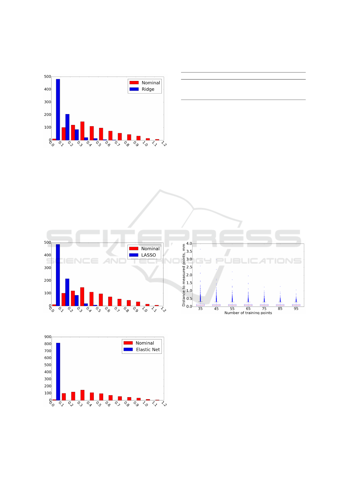
Figure 2: Frequency histogram of the distance error (mm)

for Ridge regression.

To illustrate the results of the modeling, error pa-

rameters were estimated by the trained models for the

test set and the corrected positions of the EE were cal-

culated. The frequency plot of the resulting positional

errors, measured as the distance between the nomi-

nal and measured position alongside with the distance

from modeled to measured position, for Ridge (Fig-

ure 2), LASSO (Figure 3), and Elastic Net regression

(Figure 4) shows signiﬁcant shift of error distribution

towards zero.

Figure 3: Frequency histogram of the distance error (mm)

for LASSO regression.

Figure 4: Frequency histogram of the distance error (mm)

for Elastic Net regression.

Table 2: Distance error (mm) before and after modeling.

Error Measured Modeled

Ridge LASSO Elastic Net

mean 0.48 0.11 0.11 0.03

std 0.25 0.10 0.09 0.01

max 1.17 0.68 0.54 0.06

To better compare the results of the error model-

ing, Table 2 combines the statistical information for

the modeled error parameters. A substantial decrease

in standard deviation values for all models in compar-

ison to the nominal robot values can be observed. It

can also be seen that Elastic Net regression showed

best results in comparisson to other models.

4.3 Size of the Training Set

To investigate how the size of the training set inﬂu-

ences the performance of the modeling approaches,

error models were trained using [25, 35, . . . , 95] points

from the available dataset. To ensure that each point

was used for training and testing at least once 5-fold

CV was used. To account for the variance in the algo-

rithm itself the CV procedure was run 25 times, giv-

ing an estimate of the performance of the algorithm

on the dataset and an estimation of how robust its per-

formance is.

Figure 5: Distance error for the test set for different number

of training points for Ridge regression.

The box plots of the resulting positional errors

for Ridge (Figure 5), LASSO (Figure 6), and Elastic

Net regression (Figure 7) show that the mean value

stays almost the same and only the maximum values

change. From the Table 3, that presents the statis-

tical information of the regression models comparis-

son, we can see that Elastic Net shows the best results.

5 CONCLUSIONS

A learning based approach using the Adjoint error

model and POE formula was presented and evalu-

Learning-based Kinematic Calibration using Adjoint Error Model

377

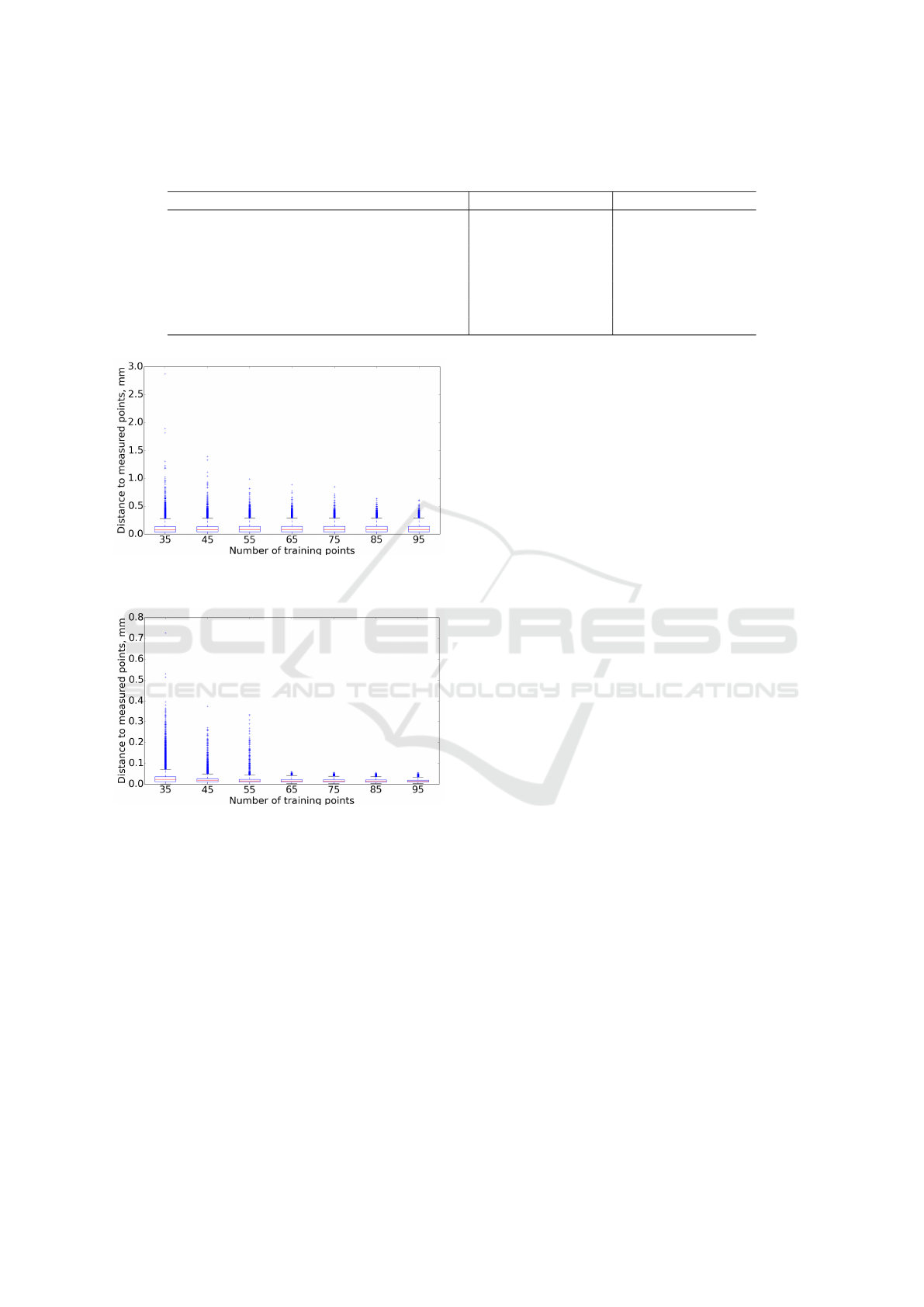
Table 3: Distance error (mm) comparisson for different sizes of training sets based on 25 repetitions.

Size of the training set Ridge LASSO Elastic Net

mean std max mean std max mean std max

35 0.12 0.12 3.65 0.10 0.09 2.87 0.03 0.03 0.72

45 0.11 0.10 2.99 0.10 0.08 1.39 0.02 0.02 0.37

55 0.11 0.09 2.22 0.10 0.08 0.99 0.02 0.01 0.33

65 0.11 0.07 1.95 0.10 0.08 0.89 0.02 0.01 0.06

75 0.11 0.08 1.25 0.10 0.08 0.85 0.01 0.01 0.06

85 0.11 0.08 1.28 0.10 0.07 0.64 0.01 0.01 0.05

95 0.10 0.08 1.07 0.10 0.07 0.61 0.01 0.01 0.05

Figure 6: Distance error for the test set for different number

of training points for LASSO regression.

Figure 7: Distance error for the test set for different number

of training points for Elastic Net regression.

ated on example of KUKA LBR iiwa 7 R800. Kine-

matic and non-kinematic inﬂuences were included in

the calibration model without explicitly using phys-

ical models, by distributing their inﬂuence over in-

troduced error parameters. Regression analysis was

then used to predict their values for new data. Three

regression methods were compared on the number

of training points and resulting distance error us-

ing a dataset containing positional measurements of

the robot ﬂange. As a result of this evaluation, all

three models showed decrease in distance errors at

the EE having low mean values over different num-

ber of training points. The Elastic Net model showed

best results by signiﬁcantly improving the absolute

accuracy of the manipulators tool position using a

model depending on nominal Cartesian position of

the EE and joint conﬁgurations of the robot. An

example model trained with 60 points reduced the

mean value of the positional errors from 0.4808 mm to

0.0337 mm and the maximum value from 1.1513 mm

to 0.0601 mm.

As any learning based approach the proposed

method highly depends on the training data. As part

of the future work inﬂuences of different input param-

eters will be evaluated by designing different experi-

ments. Another important goal is to ﬁnd some optimal

distribution and minimal number of points necessary

for training to reach needed accuracy. The dynamic

robot calibration, in which the impact of the motion

is considered, can also be applied using the proposed

method, if apropriate input parameters are used for

building the error model.

REFERENCES

Brockett, R. W. (1984). Robotic manipulators and the prod-

uct of exponentials formula. In Mathematical theory

of networks and systems, pages 120–129. Springer.

Chen, G., Wang, H., and Lin, Z. (2014). Determination of

the identiﬁable parameters in robot calibration based

on the poe formula. IEEE Transactions on Robotics,

30(5):1066–1077.

Chen, I.-M., Yang, G., Tan, C. T., and Yeo, S. H. (2001). Lo-

cal poe model for robot kinematic calibration. Mech-

anism and Machine Theory, 36(11-12):1215–1239.

Denavit, J. (1955). A kinematic notation for low pair mech-

anisms based on matrices. ASME J. Appl. Mech.,

22:215–221.

Elatta, A., Gen, L. P., Zhi, F. L., Daoyuan, Y., and Fei, L.

(2004). An overview of robot calibration. Information

Technology Journal, 3(1):74–78.

Hayati, S. and Mirmirani, M. (1985). Improving the abso-

lute positioning accuracy of robot manipulators. Jour-

nal of Robotic Systems, 2(4):397–413.

Hoerl, A. E. and Kennard, R. W. (1970). Ridge regression:

Biased estimation for nonorthogonal problems. Tech-

nometrics, 12(1):55–67.

ICINCO 2018 - 15th International Conference on Informatics in Control, Automation and Robotics

378

Klimchik, A., Furet, B., Caro, S., and Pashkevich, A.

(2015). Identiﬁcation of the manipulator stiffness

model parameters in industrial environment. Mech-

anism and Machine Theory, 90:1–22.

Li, C., Wu, Y., L

owe, H., and Li, Z. (2016). Poe-based robot

kinematic calibration using axis conﬁguration space

and the adjoint error model. IEEE Transactions on

Robotics, 32(5):1264–1279.

Liou, Y. A., Lin, P. P., Lindeke, R. R., and Chiang, H.-D.

(1993). Tolerance speciﬁcation of robot kinematic pa-

rameters using an experimental design techniquethe

taguchi method. Robotics and computer-integrated

manufacturing, 10(3):199–207.

Lorusso, A., Eggert, D. W., and Fisher, R. B. (1995). A

comparison of four algorithms for estimating 3-d rigid

transformations. In Proceedings of the British Confer-

ence on Machine Vision, pages 237–246.

Marie, S., Courteille, E., and Maurine, P. (2013). Elasto-

geometrical modeling and calibration of robot manip-

ulators: Application to machining and forming appli-

cations. Mechanism and Machine Theory, 69:13–43.

Mooring, B. (1983). The effect of joint axis misalignment

on robot positioning accuracy. In Proceedings of the

ASME International Computers in Engineering Con-

ference and Exhibition, pages 151–155.

Murray, R. M., Li, Z., Sastry, S. S., and Sastry, S. S. (1994).

A mathematical introduction to robotic manipulation.

CRC press.

Okamura, K. and Park, F. C. (1996). Kinematic calibration

using the product of exponentials formula. Robotica,

14(04):415–421.

Rawlings, J. O., Pantula, S. G., and Dickey, D. A. (2001).

Applied regression analysis: a research tool. Springer

Science & Business Media.

Tibshirani, R. (1996). Regression shrinkage and selection

via the lasso. Journal of the Royal Statistical Society.

Series B (Methodological), pages 267–288.

Zhuang, H., Roth, Z. S., and Hamano, F. (1992). A

complete and parametrically continuous kinematic

model for robot manipulators. IEEE Transactions on

Robotics and Automation, 8(4):451–463.

Zou, H. and Hastie, T. (2005). Regularization and variable

selection via the elastic net. Journal of the Royal Sta-

tistical Society: Series B (Statistical Methodology),

67(2):301–320.

Learning-based Kinematic Calibration using Adjoint Error Model

379