Extension of the Model-based Pre-step Stabilization Method for

Non-iterative Co-simulation

Including Direct-feedthrough

Simon Genser and Martin Benedikt

Virtual Vehicle Research Center, Inffeldgasse 21a, Graz, Austria

Keywords:

Pre-step Stabilization, Co-simulation, Weak Coupling, Interface Jacobians.

Abstract:

For integration of subsystems co-simulation tools and master algorithms have to cope with the problem of re-

stricted access to subsystem information. Especially for efﬁcient handling of inherent properties like stiffness

and direct feedthrough of industrial co-simulations additional subsystem information is mandatory. As pro-

vision of dedicated partial derivatives, especially regarding subsystem states, is complex and computationally

expensive, recently a novel pre-step co-simulation approach for handling stiff system simulations based on for-

mal subsystem transformations was proposed. The approach follows the idea of the Nearly Energy Preserving

Coupling Element (NEPCE) scheme where exclusively subsystem inputs are modiﬁed for compensation of the

co-simulation discretization error. This paper outlines a generalization of the presented pre-step co-simulation

method for handling stiffness and direct feedthrough of subsystems. The generalized pre-step co-simulation

algorithm is examined along a theoretical 2 DoF benchmark co-simulation example indicating outstanding

co-simulation performance.

1 INTRODUCTION

Nowadays, usage of numerical simulation for design,

analysis and engineering of technical systems is com-

mon practice in industry and a lot of different mod-

elling approaches and tailored numerical solvers are

available. When it comes to holistic system consid-

erations typically subsystem simulations from differ-

ent domains, departments or companies have to be in-

tegrated and co-simulation is the preferred solution

(Arnold, 2006). This way, subsystems are handled

as black-boxes with deﬁned interfaces for the control

and the exchange of inputs and outputs and higher-

level integration schemes are necessary for synchro-

nization purposes, i.e. master algorithms (Bastian

et al., 2011). As in classical numerical simulation

the evaluation of the right-hand side of the govern-

ing subsystem equations is crucial for efﬁcient treat-

ment of overall stiff co-simulations and related Jacobi

matrices are typically used by the master algorithm

when linear subsystem behaviour can be assumed.

Accessing subsystem model information itself has to

be supported by the simulation tools via enhanced co-

simulation capabilities or by implementation of the

Functional Mock up Interface, a standard for model

exchange and integration for data exchange and con-

trol of subsystem simulations. Especially FMI 2.0

supports the exchange of partial derivatives of sub-

system models.

Utilization of the right-hand side evaluations of sub-

systems – partial derivatives of subsystem models

- by master algorithms is beneﬁcial for improving

overall co-simulation performance and, on the other

hand, mandatory for handling dedicated properties

and characteristics of the co-simulation at hand. As

co-simulation is typically applied in cases where it is

impossible to port and assemble the individual sub-

system simulations into a standalone, multi-purpose

simulation model and its related tool, due to missing

modelling features or tailored solvers, rather complex

subsystems have to be integrated. These subsystems

most often possess properties like stiffness and direct

feedthrough.

Similar to classical numerical simulation stiffness is

addressed by implicit schemes or at least explicit

ones with implicit behavior, e.g. linearly-implicit ap-

proaches (Rosenbrock W-methods) (Cellier and Kof-

man, 2010). Direct feedthrough represents a subsys-

tem property which inﬂuences overall system stabil-

ity. Assuming the assembled overall system is stable

(Kuebler and Schiehlen, 2000), direct feedthroughs of

individual subsystems introduce proportional input-

Genser, S. and Benedikt, M.

Extension of the Model-based Pre-step Stabilization Method for Non-iterative Co-simulation - Including Direct-feedthrough.

DOI: 10.5220/0006848002230231

In Proceedings of 8th International Conference on Simulation and Modeling Methodologies, Technologies and Applications (SIMULTECH 2018), pages 223-231

ISBN: 978-989-758-323-0

223

output dependencies of subsystems, affecting per-

formance

of the master algorithms too. Some ap-

proaches are published (Arnold, 2006; Sicklinger

et al., 2013; Sadjina et al., 2016; Viel, 2014) to cope

with direct feedthrough. In contrast, recently, another

non-iterative approach was proposed based on formal

subsystem transformations and the utilization of sub-

systems Interface Jacobians exclusively, referred to as

NECPE-II (Genser and Benedikt, 2018), in order to

reduce the computational burden on subsystem side.

Within this paper the proposed algorithm is general-

ized for handling of subsystems direct feedthroughs.

The paper is organized as follows: Section 2 contains

the detailed derivation of the pre-step stabilization

algorithm. In Section 3 the improved performance

of the presented algorithm is illustrated by a 2 DoF

benchmark co-simulation example.

2 PRE-STEP ALGORITHM

The aim of this paper is to generalize the model-based

pre-step stabilization method (NEPCE-II) for the non-

iterative co-simulation (Genser and Benedikt, 2018)

in order to handle additionally direct feedthroughs of

subsystems.

2.1 System Description

The state-space representation (Dorf and Bishop,

2017) of subsystem S

˙x

(t) = A

· x

(t) + B

· u

(t) (1)

(t) = C

· x

(t) + D

· u

(t) (2)

is a suitable option to include direct feedthrough. The

condition:

6= 0,

for least an i = 1, . . . , N assures the presence of a

direct feedthrough, whereby N denotes the number

of subsystems included in the overall co-simulation.

Compared to the output-based system description in

in (Genser and Benedikt, 2018), the herein used one

(3) has an additional term, presented by ˙u

˙y

= S

, u

, ˙u

). (3)

The proposed pre-step coupling algorithm is based on

the linearization of (3) around (0, 0, 0):

˙y

≈ S

(0, 0, 0)+

∂S

∂y

· y

∂S

∂u

· u

∂S

∂ ˙u

· ˙u

Note: In the context of co-simulation, handling of direct

feedthroughs is different to handling differential algebraic

equations, as direct feedthroughs are not stating constraints

on subsystem states.

Without loss of generality one can assume that

(0, 0, 0) = 0, which leads to the transformed lin-

earized output-based subsystem description:

˙y

≈

∂S

∂y

· y

∂S

∂u

· u

∂S

∂ ˙u

· ˙u

. (4)

As complete partial-derivatives are typically difﬁcult

to be accessed, in most cases a linear approximation

of the subsystems is used. Especially this is speciﬁed

by the Functional Mock up Interface 2.0 (Blochwitz,

2012). Therefore a connection between this represen-

tation an the utilized output-based description (4) is

desirable. The derivation of this transformation starts

with the time derivative of (2):

˙y

= C

· ˙x

+ D

· ˙u

Substituting (1) leads to:

˙y

= C

· (A

· x

+ B

· u

) + D

· ˙u

. (5)

Rearranging (2) and inserting into (5) results in:

˙y

= C



·C

−1

· (y

− D

· u

) + B

· u



+ D

· ˙u

From algebraic rearrangements follows:

˙y



· A

·C

−1



· y

+ . . .

. . .



· B

−C

· A

·C

−1

· D



· u

+ D

· ˙u

Comparing this equation to (4) directly turns out the

related transformation rules

∂S

∂y

= C

· A

·C

−1

∂S

∂u

= C

· B

−C

· A

·C

−1

· D

∂S

∂ ˙u

= D

In case of black-box subsystems, system identi-

ﬁcation methods are used to approximate (4) di-

rectly. There are different system identiﬁcation meth-

ods available. The herein preferred ones, due to

their ability to identify direct feedthrough, are the

so-called subspace methods (Overschee and Moor,

1996; Trnka, 2005), especially the Multivariable

Output-Error State Space (MOESP) algorithm, see

(Katayama, 2005).

2.2 Derivation of the Algorithm

To keep the notation in the following derivation of the

algorithm as simple as possible the following assump-

tions are made:

For generalization purposes the term C

−1

represents the

pseudo-inverse.

SIMULTECH 2018 - 8th International Conference on Simulation and Modeling Methodologies, Technologies and Applications

224

• the macro-step size ∆T and the micro-step size δT

are ﬁxed for the whole computation time and for

all subsystems (i.e. ∆T

= ∆T , δT

= δT );

• the overall co-simulation consists of two fully

coupled subsystems (i.e. u

= y

, u

= y

at the

coupling instants and N = 2);

• the input and output signals u, y are scalars for

both subsystems;

• the output y describes a time continuous signal.

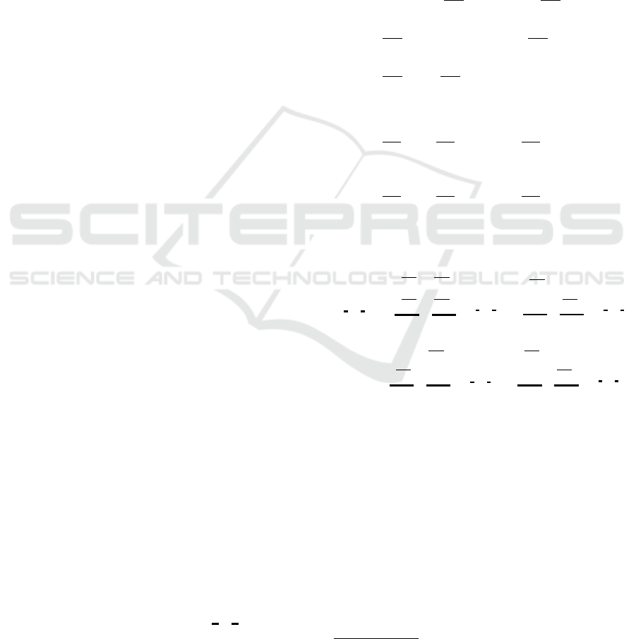
As outlined in (Genser and Benedikt, 2018) also the

generalized algorithm contains three main steps as il-

lustrated in Figure 1:

1. approximate the exact, monolithic output ˜y utiliz-

ing the global Error Differential Equation;

2. perform a global model-based extrapolation ˆy of

the output;

3. based on the extrapolation ˆy perform a local opti-

mization of the input u for every subsystem indi-

vidually.

From an abstract point of view these steps basically

comply with the ones in (Genser and Benedikt, 2018)

but differs in important details. To outline the dif-

ferences the complete derivation of the main steps is

given in the subsections below.

2.2.1 Step 1: Solving the Error Differential

Equation

To approximate the exact, monolithic solution ˜y

over

the last macro-step [T

k−1

, T

], see Step 1 in Figure 1,

of a subsystem the so-called Error Differential Equa-

tion is solved and its derivation is based on the sub-

system description (3) and two important cases:

Ideal coupling of the two subsystems:

˜y

= S

( ˜y

, ˜y

˜y

) (6)

˜y

= S

( ˜y

, ˜y

˜y

) (7)

Coupling by co-simulation:

˙y

= S

, u

, ˙u

) (8)

˙y

= S

, u

, ˙u

) (9)

Comparing (6) with (8):

˙y

− S

, u

, ˙u

) =

˜y

− S

( ˜y

, ˜y

˜y

rearranging and the deﬁnition of δ

:= ˜y

−y

, see Fig-

ure 1, leads to:

( ˜y

, ˜y

˜y

) − S

, u

, ˙u

) =

˜y

− ˙y

{z }

. (10)

Rearranging and substituting ε

:= y

− u

and

:= y

− u

, see Figure 1, into (10) leads to:

+ ε

+ δ

, y

+ δ

, ˙y

) − . . .

. . .S

+ ε

, y

− ε

, ˙y

−

)

Evaluating

the equation in T

leads to:

+ ε

+ δ

, y

+ δ

, ˙y

) − . . .

. . .S

+ ε

, y

− ε

, ˙y

−

From the spatial linearization based on the Taylor-

series, with the center of the series in (u

), y

:= y

), ˙y

:= ˙y

)) it follows

, y

, ˙y

) +

∂S

∂y

· (ε

+ δ

) +

∂S

∂u

· δ

+ . . .

. . .

∂S

∂ ˙u

− S

, y

, ˙y

) −

∂S

∂y

· (ε

) + . . .

. . .

∂S

∂u

· ε

∂S

∂ ˙u

≈

From algebraic rearrangements follows the ﬁnal ordi-

nary Error Differential Equation

≈

∂S

∂y

· δ

∂S

∂u

· [δ

+ ε

] +

∂S

∂ ˙u

· [

(11)

Via symmetry for (7) and (9) it follows:

≈

∂S

∂y

· δ

∂S

∂u

· [δ

+ ε

] +

∂S

∂ ˙u

· [

(12)

The fact that the two ordinary differential equa-

tions above are coupled motivates to write them in

vector and matrix notation





|{z}

∂S

∂y

∂S

∂u

∂S

∂u

∂S

∂y

| {z }





|{z}

=:δ

∂S

∂u

∂S

∂u

| {z }





|{z}

=:ε

∂S

∂ ˙u

∂S

∂ ˙u

| {z }





|{z}

∂S

∂ ˙u

∂S

∂ ˙u

| {z }





|{z}

Rearranging this equation leads to

(I −

C) ·

δ =

A · δ

δ +

B · ε

ε +

D ·

ε,

where I denotes an identity matrix from appropriate

dimension. With the use of the pseudo inverse (I −

−1

the ﬁnal Error Differential Equation for results

δ = (I −

−1



A · δ

δ +

B · ε

ε +

D ·



. (13)

Note: Due to the deﬁnition of δ and the assumption

that y is continuous it follows that δ is continuous as

well. This leads naturally to the initial conditions for

δ, combining this with the equation above leads to a

initial value problem for the computation of the exact

output ˜y in [T

k−1

, T

For δ

and ε

the sub index k is omitted for sake of simplic-

ity.

Extension of the Model-based Pre-step Stabilization Method for Non-iterative Co-simulation - Including Direct-feedthrough

225

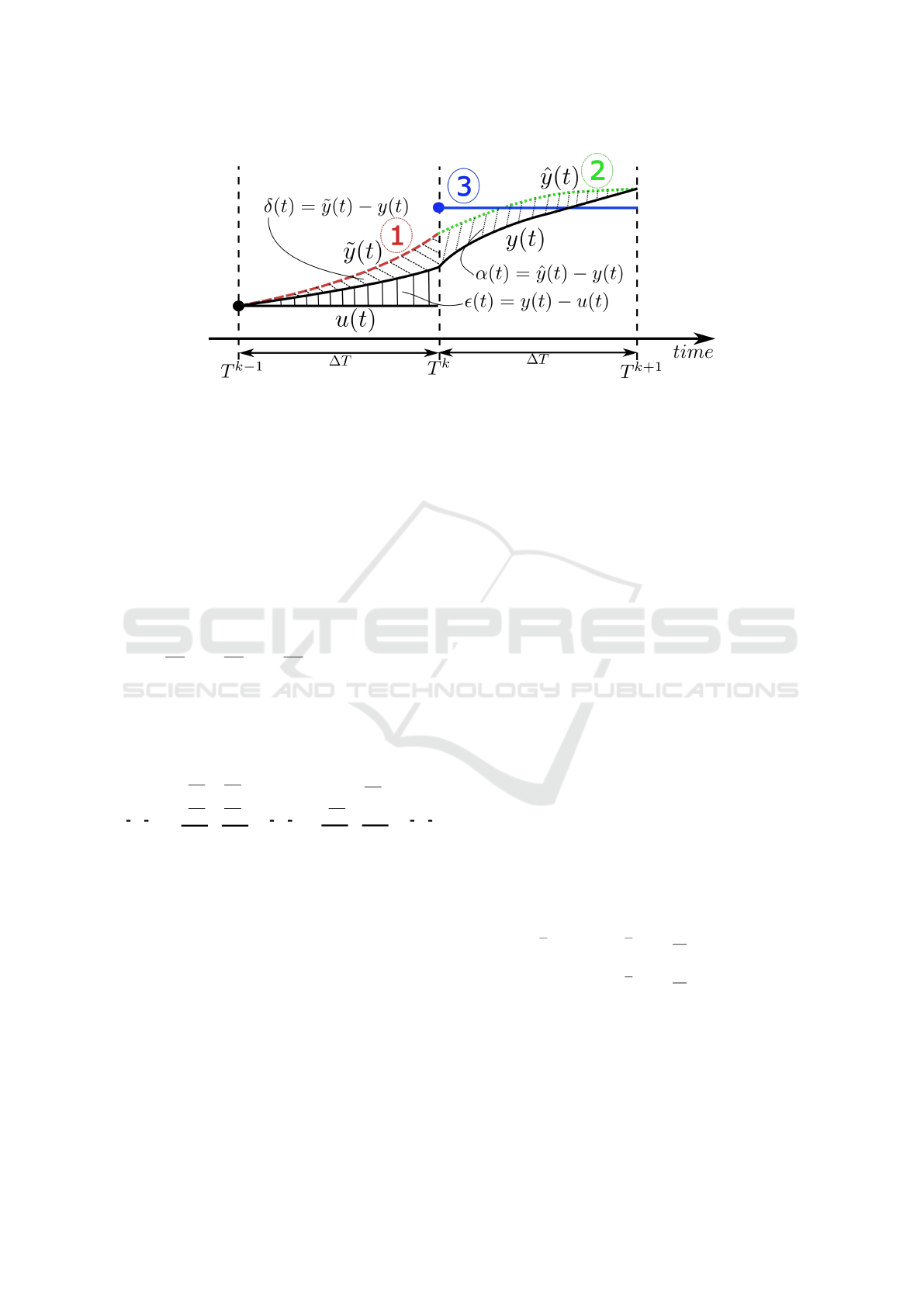
Figure 1: Illustration of the model-based pre-step stabilization algorithm (Genser and Benedikt, 2018).

2.2.2 Step 2: Model-based Extrapolation

The model-based extrapolation of the overall system

ensures the implicit behaviour of the algorithm. The

idea is to predict the future progress of the exact solu-

tion ˆy over the next macro-step ∆T , depicted as Step 2

in Figure 1. By the exact solution is the monolithic so-

lution meant, i.e. all errors due to the weak coupling

vanish. The differential equation for the extrapolation

is based on the assumption of ideal coupling between

the subsystems and the system description (4).

The derivation of the differential equation starts with

ˆy

≈

∂S

∂y

· ˆy

∂S

∂u

· u

∂S

∂ ˙u

· ˙u

for i = 1, 2. (14)

Assuming ideal coupling between subsystems

ˆy

= u

ˆy

= u

and inserting this in equation (14) leads to:



ˆy



|{z}

∂S

∂y

∂S

∂u

∂S

∂u

∂S

∂y

| {z }



ˆy



|{z}

∂S

∂ ˙u

∂S

∂ ˙u

| {z }



ˆy



|{z}

Rearranging this equation and utilizing the pseudo-

inverse (I −

−1

results in the ﬁnal differential equa-

tion:

y = (I −

−1

A ·

y. (15)

Note: The initial condition for (15) comes from

the solution of the Error Differential Equation, i.e.

ˆy(T

) = ˜y(T

) for the extrapolation over [T

, T

k+1

leading to a initial value problem for every macro time

step.

2.2.3 Step 3: Pre-step Input Optimization

The local optimization of the input u

represents the

third main part of the presented algorithm, for illus-

tration see Figure 1. Local means that this part can be

computed for every subsystem individually and inde-

pendent from the other subsystems, therefore the sub

index i is omitted in this subsection. The optimization

is based on the error:

α := ˆy − y. (16)

The idea is to choose the input u so that α is mini-

mized over the next macro-step:

min

t∈[T

k+1

]

|α(t)| (17)

There are different ways to solve the optimization

problem (17), herein the focus lies on a discretized

solution, based on the macro-step, i.e. (17) is trans-

formed into:

|α

k+1

= 0, with α

k+1

:= α(T

k+1

) (18)

The discretization (18) of the optimization problem

leads, with the deﬁnition (16), to

ˆy

k+1

= y

k+1

, (19)

where ˆy

k+1

:= ˆy(T

k+1

) and y

k+1

:= y(T

k+1

). For ex-

plicitly solving this problem the dependency of the

output y

k+1

on the input u

has to be exploited. To

describe this relation a close look on the system de-

scription (4) and standard theory of ordinary differen-

tial equations is needed. The analytical solution of (4)

is described through:

y(t) = e

∂S

∂y

·t

· y

start

∂S

∂y

·(t−τ)

∂S

∂u

· u(τ) dτ + . . .

. . .

start

∂S

∂y

·(t−τ)

∂S

∂ ˙u

· ˙u(τ) dτ,

(20)

where y

denotes the initial condition. The derivative

˙u denotes the classical time derivative which is com-

puted piecewise for every macro-step. Due to the ap-

pearance of ˙u in (20) the choice of piecewise constant

basic functions is a bad one because ˙u would be zero

all the time and so the second integral in (20) would

SIMULTECH 2018 - 8th International Conference on Simulation and Modeling Methodologies, Technologies and Applications

226

be always neglected and this would lead to a worse

approximation. That is the reason that piecewise lin-

ear basic functions are utilized to describe the input u

in the following, i.e. the preferred approach for u is

u(t) = u

+ s

·t for t ∈ [T

, T

k+1

], (21)

where u

= y(T

), with y representing the output from

the coupled subsystem. The slope of u in the macro-

step [T

, T

k+1

] is denoted with s

. Inserting this ap-

proach in (20) leads to

y(t) =e

∂S

∂y

·t

· y

∑

l=0

l+1

∂S

∂y

·(t−τ)

∂S

∂u

· . . .

. . .(u

+ s

· τ) dτ +

∑

l=0

l+1

∂S

∂y

·(t−τ)

∂S

∂ ˙u

· s

dτ.

The separation and summation of the integrals in the

macro-steps is necessary due to the piecewise deﬁni-

tion of u in (21). With T

= t

start

the starting time of

the overall co-simulation is denoted and for the lack

of simplicity ∆T and k are chosen so that T

k+1

= t

holds. Rearranging the last equation results in

y(t) = e

∂S

∂y

·t

· y

∑

l=0

l+1

∂S

∂y

·(t−τ)

∂S

∂u

dτ + . . .

(22)

. . .

∑

l=0

l+1

∂S

∂y

·(t−τ)

∂S

∂u

· τ dτ + . . . (23)

. . .

∑

l=0

l+1

∂S

∂y

·(t−τ)

∂S

∂ ˙u

dτ, (24)

with

(t) := e

∂S

∂y

·t

(t) :=

l+1

∂S

∂y

·(t−τ)

∂S

∂u

dτ,

(t) :=

l+1

∂S

∂y

·(t−τ)

∂S

∂u

· τ dτ,

(t) :=

l+1

∂S

∂y

·(t−τ)

∂S

∂ ˙u

dτ,

it is possible to write the analytic solution of y as

y(t) = φ

(t) · y

∑

l=0

· φ

(t) + . . .

. . . s



(t) + φ

(t)



. (25)

To fulﬁl (19) it is necessary to evaluate (25) in T

k+1

this leads to

k+1

= φ

k+1

) · y

∑

l=0

· φ

k+1

) + . . .

. . .

∑

l=0



k+1

) + φ

k+1

)



Recursive inserting of the equation above leads to

k+1

=φ

(∆

) · y

+ u

· φ

k+1

) + . . .

. . .s



k+1

) + φ

k+1

)



. (26)

Remark: φ

(∆

), φ

k+1

), . . . , φ

k+1

) denote

matrices with constant coefﬁcients. Similar to the

transitions matrices for the standard state-space rep-

resentation see (Dorf and Bishop, 2017).

Therefore (26) can be seen as an algebraic computa-

tion equation, the time variable and the sub index k

are omitted, denoted as

k+1

= φ

· y

+ φ

· u

+ s

· (φ

+ φ

). (27)

Inserting (27) into (19) results in

ˆy

k+1

= φ

· y

+ φ

· u

+ s

· (φ

+ φ

) (28)

As it is the case, that y

and u

is known from the pre-

vious macro time increment and ˆy

k+1

is given due to

the extrapolation, see Section 2.3.2, it is now possible

to determine s

through

= (φ

+ φ

)

−1



ˆy

k+1

− φ

· y

+ φ

· u



. (29)

It should be mentioned that, this input optimization

is computed locally and can therefore be easily per-

formed in parallel.

Remark: Comparing this derivation herein with the

basic algorithm in (Genser and Benedikt, 2018) leads

to the conclusion that a direct feedthrough in a sub-

system leads to additional terms in the subsystem de-

scription, see (4). These additional terms are the rea-

son for the differences in the derivation of the three

main steps. Setting the direct feedthrough terms to

zero, the algorithm is exactly the same as in the one

in (Genser and Benedikt, 2018), therefore the herein

presented method is a true generalization of model-

based pre-step stabilization. The generalization of

this algorithm to a co-simulation consisting of more

than two subsystems is straightforward, utilizing the

coupling matrix L (L · y = u) properly.

3 THEORETICAL EXAMPLE

To illustrate the improved performance of the herein

presented algorithm a force-displacement coupled

two-degrees of freedom oscillator has been chosen,

see (Benedikt et al., 2013; Busch, 2012). The classi-

cal First-Order-Hold (FOH), the linearly-implicit sta-

bilization (Arnold, 2011) and the energy-preserving

approach (NEPCE) (Benedikt and Hofer, 2013) are

utilized to compare the presented pre-step coupling

algorithm with state of the art methods.

Extension of the Model-based Pre-step Stabilization Method for Non-iterative Co-simulation - Including Direct-feedthrough

227

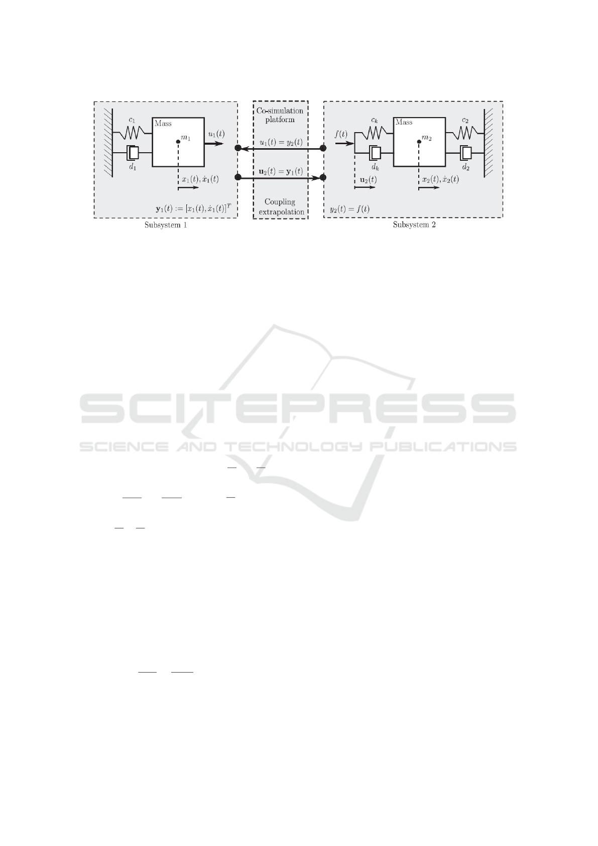
Figure 2: Co-simulation setup of a coupled 2-DOF oscillator, see (Benedikt et al., 2013).

3.1 Two Degree-of-Freedom Oscillator

The preferred example represents a two degree-of-

freedom (DoF) mechanical oscillator and is sepa-

rated into two subsystems (Fig. 2), including a direct

feedthrough in the second subsystem; the state-space

representation of the subsystems is given by:

= A

· x

+ B

· u

, (30)

= C

· x

(31)

and

= A

· x

+ B

· u

, (32)

= C

· x

+ D

· u

(33)

with



˙x



, x



˙x



, A



0 1

−





0 1

−



, B







0 0



, C



1 0

0 1







, D



−c

−d



Choosing parameters like:

= 10 kg, m

= 10 kg, c

= 10

−1

= 10

−1

, d

= 1 Nsm

−1

, d

= 2 Nsm

−1

= 10

−1

, d

= 10

Nsm

−1

start

= 0, t

end

= 0.5,

results in an overall stiffness:

max

min

−10

−50

= 200.

The initial conditions are set to:

= 0.1, ˙x

= 0, x

= 0, ˙x

= 0. (34)

The constant macro-step size is varied for evalua-

tion purposes within the interval ∆T ∈ [10

−5

, 8·10

−3

];

the ﬁxed micro-step size is set to δT = 10

−5

. The ref-

erence solution y

re f

is determined individually by uti-

lizing a monolithic simulation with ∆T = δT . There-

fore, the monolithic overall system is derived from the

subsystem description (30)-(33) assuming ideal cou-

plings u

= y

and u

= y







+ B

· D

·C







The numerical reference solution is determined by us-

ing the explicit Euler method.

3.2 Performance Evaluation

For comparison purposes the following Figures 3 to 7

illustrate the force coupling variable y

(t) exchanged

between the two subsystems.

In a ﬁrst aspect the impact of utilizing piecewise lin-

ear (Fig. 3) or piecewise constant basis functions (Fig.

4) for the extrapolated inputs is examined. By com-

paring both ﬁgures piecewise constant basis functions

leads to increased co-simulation discretization errors.

The signiﬁcant discontinuous steps in the force signal

at coupling time instances are caused by the steps in

the input signal and the existing direct feedthrough

6= 0) in Subsystem 2. A second reason of us-

ing piecewise linear basis functions is motivated by

the generalization of the pre-step stabilization method

where the time derivative of the input ˙u appears, e.g.

see (4) and (13). As the usage of piecewise constant

basis functions ( ˙u = 0) will eliminate the generalized

terms piecewise linear basis functions have been used

for the following computations.

With respect to the classical NEPCE method, in con-

trast to piecewise linear functions (Fig. 5 ), piecewise

constant functions (Fig. 6) indicate improved stabil-

ity. In case of classical NEPCE applications piece-

wise constant functions are utilized for comparison.

SIMULTECH 2018 - 8th International Conference on Simulation and Modeling Methodologies, Technologies and Applications

228

Figure 3: ∆T = 0.002; output y

by FOH input extrapola-

tion.

Figure 4: ∆T = 0.002; output y

by ZOH input extrapola-

tion.

In Figure 5 y

is illustrated for a macro step-size of

∆T = 0.00305, which indicates the stability border

of the FOH coupling approach. Figure 6 illustrates

results for ∆T = 0.0037 and indicates the stability

border of the NEPCE coupling (Benedikt and Hofer,

2013). The stability limit of the linearly-implicit sta-

bilization (Arnold, 2011) is experimentally deterem-

ined at a macro-step-size of ∆T = 0.008, see Fig. 7.

By considering all cases, Fig. 5 to 7, the herein pre-

sented pre-step stabilization method outperforms state

of the art algorithms, also in the case of eventually ex-

isting direct feedthroughs in subsystems.

For pointing out the signiﬁcantly improved stability

behavior of the proposed pre-step stabilization algo-

rithm in detail, a logarithmic error plot, depending on

the macro step-size ∆T is depicted in Figure 8. For

deﬁning a meaningful error measure, the following

relative error is introduced:

err :=

∑



norm

· max

t∈[t

start

end

]

re f

(t) −y

(t)|



(35)

with

norm

:= max

t∈[t

start

end

]

re f

(t)] − min

t∈[t

start

end

]

re f

(t)].

As the different outputs may vary in their magnitudes

the constant norm

, describing the ranges of the out-

puts y

, is introduced for normalization purposes in

Figure 5: Output y

; stability border ∆T = 0.00305 for FOH

coupling; NEPCE solution with FOH.

Figure 6: Output y

; stability border ∆T = 0.0037 for

NEPCE coupling (Benedikt and Hofer, 2013); NEPCE so-

lution with ZOH.

Figure 7: Output y

; stability border ∆T = 0.008 for linear

implicit stabilization coupling (Arnold, 2011).

(35). It is worthy to mention that in the computation

of the error depicted in Figure 8 all three different out-

puts (y

, y

) of the subsystems are considered. As one

is interested to analyze the stability of the different

coupling algorithms the simulation time is extended

to t

end

= 0.5 s, so instabilities which are growing over

the time are higher weighted. Figure 8 turns out fol-

lowing conclusions:

• an improved stability of the pre-stabilization ap-

proach using piecewise linear functions (FOH)

is pointed out within the interval of ∆T ∈

[10

−4

, 10

−2

] compared to classical FOH, NEPCE

and the linearly-implicit couplings.

Extension of the Model-based Pre-step Stabilization Method for Non-iterative Co-simulation - Including Direct-feedthrough

229

Figure 8: Logarithmic error plot.

• a signiﬁcantly improved stability of the pre-

stabilization approach using piecewise linear

functions (FOH) is conﬁrmed within the inter-

val of ∆T ∈ [10

−4

, 10

−2

], compared to the pre-

stabilization approach using piecewise constant

functions (ZOH).

• compared to FOH, NEPCE coupling and the

linearly-implicit stabilization the pre-step stabi-

lization approaches (ZOH and FOH) are stable for

macro-step sizes about 10

−2

, as depicted in Figure

7 for ∆T = 0.008.

• the analyzed coupling algorithms behave similar

within the interval of ∆T ∈ [10

−5

, 10

−4

] where the

error is dominated by the ﬁxed micro-step size, cf.

error estimation in (Arnold, 2006).

• the difference between the pre-step stabilization

with ZOH and FOH within the interval of ∆T ∈

[10

−5

, 10

−4

] is noticeable; to be investigated in fu-

ture work.

4 CONCLUSIONS

Direct feedthroughs of subsystems degrade co-

simulation performance in general. This paper

presents an extension to a recently proposed pre-step

coupling algorithm for incorporation of optionally ex-

isting direct feedthroughs of subsystems. Due to the

extended system description the time derivative of

corresponding subsystem inputs appears, to be han-

dled additionally by the master algorithm. In contrast

to existing state of the art approaches, examination

of the algorithm along a typical used co-simulation

benchmark example turns out an outstanding perfor-

mance in terms of stability and accuracy. This signiﬁ-

cant performance improvement is justiﬁed by the pre-

step compensation of the co-simulation discretization

error based on the approximated exact solution, i.e.

the inputs to subsystems are modiﬁed according sub-

system properties like stiffness and direct feedthrough

prior to the execution of the co-simulation time incre-

ment.

5 FUTURE WORK

The current version of the pre-step co-simulation al-

gorithm is able to cope with subsystem properties like

stiffness and direct feedthrough. An extension of the

algorithm is necessary for efﬁciently handling sub-

systems described by differential algebraic equation

(DAEs), where inputs affect subsystem-internal alge-

braic constraints and thus introduce so-called drift ef-

fects. Furthermore, this contribution focusses on sub-

systems with a relative degree of zero and one. Future

research has to investigate the importance of the rela-

tive degree in the context of co-simulation. Finally,

the proposed pre-step co-simulation algorithm will

be implemented prototypically into the co-simulation

platform Model.CONNECT

T M

from AVL to be ap-

plied to realistic industrial use-cases for an extended

performance evaluation.

REMARK PATENT

The presented work describes an extension to a novel

coupling approach for co-simulation of distributed

SIMULTECH 2018 - 8th International Conference on Simulation and Modeling Methodologies, Technologies and Applications

230

dynamical subsystems. Protected by a pending Euro-

pean patent (Benedikt and Genser, 2018) the outlined

schemes are supported by the co-simulation platform

Model.CONNECT

T M

(AVL, 2018) from AVL.

ACKNOWLEDGEMENTS

The publication was written at VIRTUAL VEHI-

CLE Research Center in Graz, Austria. The authors

would like to acknowledge the ﬁnancial support of

the COMET K2 Competence Centers for Excellent

Technologies Programme of the Federal Ministry for

Transport, Innovation and Technology (bmvit), the

Federal Ministry for Digital, Business and Enterprise

(bmdw), the Austrian Research Promotion Agency

(FFG), the Province of Styria and the Styrian Busi-

ness Promotion Agency (SFG).

REFERENCES

Arnold, M. (2006). Multi-rate time integration for large

scale multibody system models. IUTAM Symposium

on Multiscale Problems in Multibody System Con-

tacts.

Arnold, M. (2011). Numerical stabilization of co-

simulation techniques, the ODE case. Martin

Luther University Halle-Wittenberg NWF II-Institute

of Mathematics.

AVL (2018). Model.connect

T M

, the neutral model inte-

gration and co-simulation platform connecting virtual

and real components. http://www.avl.com/-/model-

connect-. [Online; accessed 31.01.2018].

Bastian, J., Glau, C., Wolf, S., and Schneider, P. (2011).

Master for co-simulation using fmi. 8th Modelica

Conference, Dresden, Germany,.

Benedikt, M. and Genser, S. (2018). Pre-step co-simulation

method and device (ﬁled).

Benedikt, M. and Hofer, A. (2013). Guidelines for the ap-

plication of a coupling method for non-iterative co-

simulation. IEEE, 8th Congress on Modelling and

Simulation (EUROSIM), Cardiff Wales.

Benedikt, M., Watzenig, D., and Hofer, A. (2013). Mod-

elling and analysis of the noniterative coupling pro-

cess for cosimulation. TaylorFrancis.

Blochwitz, T. e. a. (2012). Functional mockup interface 2.0:

The standard for tool independent exchange of simu-

lation models. 9th International Modelica Conference

Munich.

Busch, M. (2012). Zur Efﬁzienten Kopplung von Simula-

tionsprogrammen. PhD thesis, University Kassel.

Cellier, F. and Kofman, E. (2010). Continuous System Sim-

ulation. Springer, New York, 1st edition.

Dorf, R. C. and Bishop, R. H. (2017). Modern Control Sys-

tems. Pearson, USA, 13th edition.

Genser, S. and Benedikt, M. (2018). Model-based pre-step

stabilization method for non-iterative co-simulation.

IMSD, Tecnico Lisboa.

Katayama, T. (2005). Subspace Methods for System Iden-

tiﬁcation. Springer-Verlag London Limited, London,

1st edition.

Kuebler, R. and Schiehlen, W. (2000). Modular simulation

in multibody system dynamics. Kluwer Academic

Publishers.

Overschee, P. V. and Moor, B. D. (1996). Subspace Iden-

tiﬁcation for Linear Systems. Kluwer Academic Pub-

lishers, London, 1st edition.

Sadjina, S., Kyllingstad, L., Skjong, S., and Peder-

sen, E. (2016). Energy conservation and power

bonds in co-simulations: non-iterative adaptive step

size control and error estimation. arXiv preprint

arXiv:1602.06434.

Sicklinger, S., V., B., and B., E. (2013). Interface-jacobian

based co-simulation. NAFEMS World Congress 2013.

Trnka, P. (2005). Subspace identiﬁcation methods.

Viel, A. (2014). Implementing stabilized co-simulation of

strongly coupled systems using the functional mock-

up interface 2.0. 10th International Modelica Confer-

ence,Lund, Sweden.

Extension of the Model-based Pre-step Stabilization Method for Non-iterative Co-simulation - Including Direct-feedthrough

231