Registration of Inconsistent Point Cloud Maps with Large Scale

Persistent Features

Simon Thompson, Masahi Yokozuka and Naohisa Hashimoto

Smart Mobility Research Group, Robot Innovation Research Center,

National Institute of Advanced Industrial Science and Technology, Tsukuba, Japan

Keywords:

Point-Cloud Registration, Inconsistent Maps.

Abstract:

Accurate point cloud registration techniques such as Iterative Closest Point matching have been developed to

produce large scale 3D maps of the environment. Typically they iteratively register point clouds captured from

adjacent sensor scans resulting in point clouds which are largely consistent. However, merging two seperate

point cloud maps constructed at different times can lead to signiﬁcant inconsistencies between the point clouds.

Existing point based registration techniques can be sensitive to local minima caused by such inconsistencies.

Feature based approaches can overcome local minimum but are typically less accurate, and can still suffer

from correspondence errors. We introduce Large Scale Persistent Features (LSPFs), sub regions of point

clouds that have orthogonal planar regions that are consistent and persist over a large spatial area. Each LSPF

is used to calculate an individual transformation estimate using traditional registration techniques. Sampling

Consensus is then used to select the best transform which is used for registration, avoiding local minima. LSPF

registration is applied to simulated point cloud maps with known inconsistencies and shown to perform with

more accuracy and lower computation time than other popular approaches. In addition, real world registration

results are presented which demonstrate LSPF registration between MMS maps and low cost sensor maps

captured 6 months apart.

1 INTRODUCTION

Accurate registration of two or more point clouds is

required to produce large scale 3D maps of the en-

vironment (Pyvanainen et al., 2012)(Shiratori et al.,

2015). Point matching based cloud registration

techniques, such as Iterative Closest Point (ICP)(Besl

and McKay, 1992) typically asumme that point cloud

data is captured from spatially and temporally close

view points, such as consecutive scans of a LIDAR

sensor mounted on a moving vehicle (Lu and Milios,

1997). Under this assumption the environment surfa-

ces which the point cloud represents do not drastically

change between view points and are generally con-

sistent. However, in some applications, such as mer-

ging two seperately constructed maps, the assumption

of temporal and spatial proximity in point cloud cap-

ture is invalid. In particular, a large temporal distance

between point cloud capture can result in signiﬁcant

changes in the environment due to factors such as

seasonal variance in vegetation or new construction.

This can lead to large inconsistencies (with a non-

random distribution) between the point clouds which

can cause the registration process to incorrectly con-

verge in local minima. (Thompson et al., 2016) report

inconsistencies when merging maps made from low

cost sensors (Yokozuka et al., 2015) with high resolu-

tion (Tao and Li, 2007) maps captured months apart.

Feature based registration approaches can over-

come local minimum but are typically less accurate,

can suffer from correspondence errors, and gene-

rally require a subsequent ﬁne grained alignment step.

This work proposes Large Scale Persistent Features

(LSPF) based registration which seeks to overcome

local minima problems while still producing the accu-

rate alignment results typical of point cloud matching

methods. LSPF are sub regions of point clouds that

consist of orthogonal planar regions that persist over

a large spatial area. A number of LSPF are detected

in the target point cloud and individual alignment is

performed on each LSPF and their associated point

cloud sub-region. Sampling Consensus is then used

to select the registration transform which has the most

support. In this way, sub-regions which are inconsis-

tent with the majority of the map can be ignored and

local minima in the registration process avoided.

The LSPF registration process is shown to be sig-

niﬁcantly faster than simple ICP matching, even when

274

Thompson, S., Yokozuka, M. and Hashimoto, N.

Registration of Inconsistent Point Cloud Maps with Large Scale Persistent Features.

DOI: 10.5220/0006847602740282

In Proceedings of the 15th International Conference on Informatics in Control, Automation and Robotics (ICINCO 2018) - Volume 2, pages 274-282

ISBN: 978-989-758-321-6

including the cost of feature detection. Simulation re-

sults show that LSPF registration can more accurately

approaches. Real world registration results are pre-

sented which demonstrate LSPF registration between

MMS maps and low cost sensor based maps captured

6 months apart.

The rest of the paper is organised as fol-

lows: Section 2 describes related work in this ﬁeld.

Section 3 describes LSPFs, how they are detected

in point clouds, and how they are used for registra-

tion. Section 4 describes a simulated environment

with known inconsistencies, and presents registration

results evaluating accuracy and computation time for

LSPF registration in comparison with other popular

approaches. Section 5 then presents some registration

results from a real world environment, and also the

results from an online data set. Finally Section 6 con-

cludes with some dicussion and introduces avenues

for further work.

2 RELATED WORK

The Iterative Closest Point (ICP) algorithm (Besl and

McKay, 1992) is a popular technique to align refe-

rence and input point clouds in a common frame of

reference. In it, corresponding points pairs between

the point clouds are indentiﬁed by closest Euclidean

distance, and then a rigid transformation is calculated

which minimises the distance between the correspon-

ding points. The estimated transform is then applied

to the input cloud to align it with the reference cloud.

This process of ﬁrst matching corresponding points

and then aligning the clouds is repeated until the alig-

nment is sufﬁciently accurate to meet some conver-

gence criterion.

ICP can produce accurate alignment results but

can be sensitive to local minimum in the convergence

basin. (Besl and McKay, 1992) state that a global mi-

nima can be reached if individual instances of ICP are

applied within each local convergence basin, though

note the computational challenges this implies. One

source of local minimima is due to the interaction

between the distribution of points on the underlying

surfaces and the choice of correspondence matching

metric. Variants of ICP such as Point-to-Plane ICP

(Chen and Medioni, 1991), and Generalised ICP (Se-

gal et al., 2009) improve stability and speed of conver-

gence by using more sophisticated matching metrics.

Another, more pernicious source of local minima

is inconsistency between the point clouds due to noise

in sensor data, or differences in the underlying surfa-

ces. To overcome this, various methods to indentify

Figure 1: Registration using multiple sub-regions of point

clouds.

inconsistent correspondence points have been propo-

sed such as Trimmed ICP (Chetverikov et al., 2002),

or RANSAC based correspondence rejection (Holz

et al., 2015). In these methods, correspondence points

determined to be inconsistent are discarded as outliers

before alignment is performed. (Gelfand et al., 2003)

propose ﬁltering points based on their stability in the

registration task. Only points whose local area covari-

ance matrix suggests good alignment information are

used in the registration process. These methods can

be computationally expensive and are still susceptible

to large non-random inconsistencies.

Feature based registration methods identify key

points in the data on which correspondence mat-

ching and outlier removal are performed. This re-

duced correspondence set can be used to calculate a

rough initial alignment which avoids local minima. A

ﬁne grained point based registration can then applied.

(Holz et al., 2015) describe various feature descrip-

tors which encode information at keypoints (Harris

and Stephens, 1988) about the local surface curva-

ture and point distribution to improve correspondence

matching. FPHF (Rusu et al., 2009) calculate des-

criptors at different scales to measure persistence of

features over spatial extent. Feature descriptor mat-

ching however can still suffer from data association

errors in both highly structured and unstructured en-

vironments.

(Weber et al., 2010) proposes sharp features which

use Gauss maps of local surface curvature to identify

regions in point clouds with strong peaks in curavture

space. This work proposes Large Scale Persistent Fe-

atures which extend the notion of sharp features to

include checking local consistency and persistence

over larger regions. Local point cloud sub-regions

around features are registered individually using ex-

isting point based techniques, avoiding both feature

decriptor based correspondence errors and the inﬂu-

ence of non-local minima. This idea is illustrated

in Figure 1, with multiple sub-regions of the point

clouds (shown in cricles) each being aligned indvi-

dually. Consensus Sampling is then applied to the set

of alignment transformations generated by the LSPFs

and the most consistent transformation is used to re-

gister the point clouds.

Registration of Inconsistent Point Cloud Maps with Large Scale Persistent Features

275

3 LARGE SCALE PERSISTENT

FEATURES

LSPFs attempt to identify sub regions of the point

cloud whose underlying surfaces provide strong cues

for registration, and are also likely to be persistent

spatially and temporally. It is assumed regions that

have mulitple (ideally orthogonal) planar components

whose structure remains consistent over a large area

satisfy these requirements. LSPF achieve this by

analysing the Normal Density Distribution (NDD) of

each sampled sub region. Structural consistency over

space is determined by the degree to which the NDD

of a sub-region remains stable as the size of the re-

gion is varied. Strong peaks in the NDD represent

planar surfaces and the distance between peaks can

determine the relative angle between planar compo-

nents. Initially a point is randomly sampled from the

cloud. This represents the center of a potential LSPF.

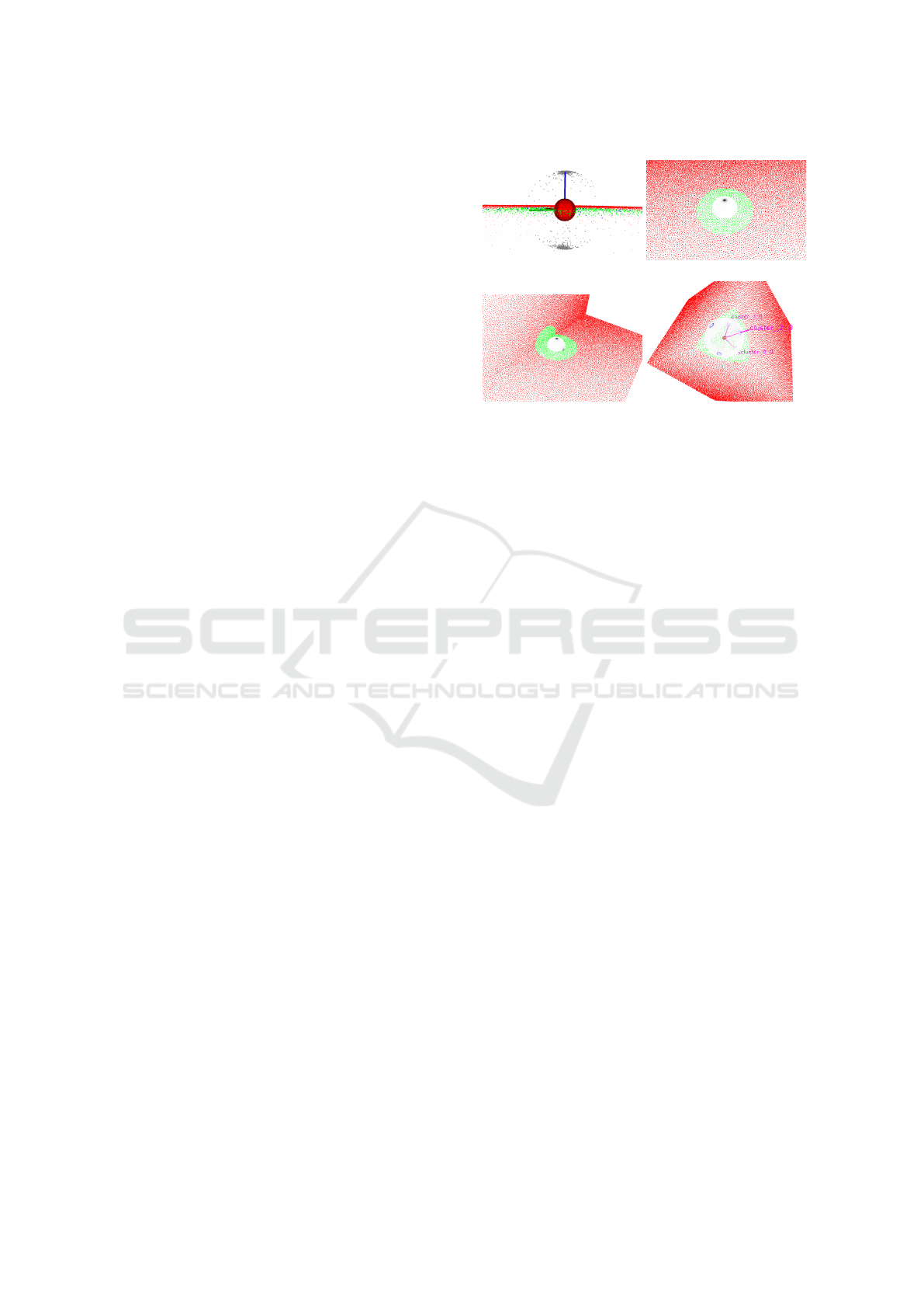
3.1 Normal Density Distribution

Given a candidate feature point, the NDD of the sur-

rounding area is calculated. Points within a given ra-

dius (2m) are randomly sampled. For each of the se-

lected points we use nearest neighbour search to ﬁnd

all points within a radius (0.3m) and randomly sam-

ple triples of points within. The triples are used to

calulate normals (vectors perpendicular to the plane

deﬁned by the three points) of the selected points.

Each normal is plotted on a unit sphere to give an

Extended Gauss Map of the local surface. The Gauss

Map for a candidate feature point on a single planar

surface is shown in Figure 2 a). The grey points show

the normals on the unit sphere centered on the can-

didate feature point (large red sphere), with normals

concentrated at opposite points on a line perpedicular

to the plane. To calculate the density of the normal

distribution over the unit shere, we ﬁrst discretise the

sphere using a Fibonnaci Lattice (N = 10000). For

each point in the Lattice, we then count the number

of normals which lie within a given radius, giving the

normal density distribution of the candidate LSPF. Fi-

gures 2 b) and c) show the NDD for features contai-

ning one and two planar surfaces respectively. Red

points show the whole point cloud map, green points

lie within the radius of the candidate LSPF, while

the NDD is drawn on the unit sphere centered on the

LSPF, with dark regions being more dense.

3.2 Centering of LSPFs

Because it is assumed persistent features maintain a

consistent NDD while varying the size of the feature,

a) b)

c) d)

Figure 2: LSPF detection: a) Gauss map of local surface

normals, b) Normal Density Distribution (NDD) for one and

c) two planes, and d) NDD clustering for corner of a cube.

surface discontinues (edges or corners) must be cente-

red within the LSPF. To achieve this, when sampling

normals, the distance of the plane deﬁned by the nor-

mal to the candidate feature point is calculated. By

averaging the resulting vectors, a vector which shifts

the center of the feature to the point of maximal sur-

face discontinuity is calculated. Iteratively shifting

the feature center by this vector (multipled by a gain

factor) moves the LSPF to the center of the local sur-

face discontinuities, supressing non-maximal feature

detection.

3.3 Growing Feature Regions

Once a feature is centered, the area covered by the

feature is grown to test the persistence of the feature

over space. By comparing the evolution of the NDD

as the feature region grows, the consistency of the un-

derlying surface structure can be evaluated. In this

work we grow the feature radius by 0.2m each step,

continuously sampling normals from the expanding

regions and updating the NDD of the feature. Change

in NDD is determined by the Sum of Absolute Dif-

ferences between the normalised NDD of the initial

region and that of the expanded region. When this

difference reaches a threshold (experimentally deter-

mined), growth is terminated.

3.4 Clustering Normals

Once a LSPF has been centered and grown, the do-

minant planes in the underlying surface are identiﬁed

by clustering peaks in the NDD. Using the density of

normals discretised by the Fibonacci Lattice, the Den-

sity Based Spatial Clustering with Noise (DBSCAN)

ICINCO 2018 - 15th International Conference on Informatics in Control, Automation and Robotics

276

algorithm is applied. Detected clusters are merged ac-

cording to the angle between cluster centroids, mer-

ging those whose centroids are less than a threshold

angular distance apart, as well as clusters lying on

opposite sides of the unit sphere. The centroids and

density of the remaining clusters form part of the re-

presentation of the LSPF. Figure 2 d) shows an exam-

ple of clusters detected on the corner of a surface with

3 planes.

3.5 LSPF Coverage

Due to the computational expense in caculating

LSPFs, an exhaustive evaluation of possible features

over the entire point cloud is impractical. Instead,

a sampling based approach is used. Random points

are iteratively selected and if the point does not lie

within the area covered by an existing feature, the

above LSPF detection method is applied. A measure

of the ratio between points sampled that lead to new

features and those that lie within previously identiﬁed

features, is used as the termination condition of the

sampling loop. In this way, sampling continues until

95 percent of sampled points lie within regions cove-

red by LSPF’s.

3.6 LSPF Suitability Measure

LSPFs represent persistent spatial structure in the en-

vironment. For the registration task, structures with

mutiple planar components that extend over a large

region are particularly useful. Here, we propose a me-

asure of how suitable a LSPF is for registration based

on density and orthogonality of the top three clusters.

The ratio of the sum of the density within the top three

clusters compared to the total sum of the density over

the entire Fibonacci Lattice give an indication of the

strength the top three features. Additionally, relati-

vely equal density among the top three clusters repre-

sents multiple planar components, while a single do-

minant density reﬂects a single plane. Formally, the

measure l of the suitability of of LSPF for registration

is given by:

l =

D(C

) + D(C

)

∑

100

i=1

D( f l(i))

∗

D(C

)

D(C

)

∗ α ∗ w

(1)

where, D(C

) is the density of cluster j, D( f l(i)) is

the density in the Fibbinoci Lattice i and w

o is a

weight proportional to the radius of the feature. And

α represents the orthognality between the cluster cen-

troids:

α = (1−(v

· v

))∗(1−(v

· v

))∗(1−(v

· v

))

(2)

where v

is the centroid vector of cluster i.

3.7 Registration with LSPFs

Given two point clouds (target and input) and an ini-

tial guess of the transformation between them, the ty-

pical registration task is to calculate the transforma-

tion that, when applied to the input cloud, optimally

aligns the two point clouds. To perform registration

with a set of LSPFs, a transformation estimation al-

gorithm is individually applied to the point cloud de-

ﬁned by each LSPF (all using the same frame of re-

ference and the same initial transformation estimate).

For each LSPF, the registration process produces an

individual transformation estimate. A sampling con-

sensus algorithm then is applied to chose the transfor-

mation estimate with the most support. In this way,

LSPFs representing regions of the point clouds which

share a common transformation contribute to the re-

gistration task, while regions with features which re-

present inconsistencies can be avoided.

In this work, we apply the well known Iterative

Closest Point registration method to estimate trans-

formations between LSPF regions, although any point

cloud based method could be used.

4 SIMULATION RESULTS

In this section we present registration results when ap-

plying LSPFs to simulated point cloud data, to con-

ﬁrm the ability of the approach to avoid errors in the

registration of point cloud data with inconsistencies.

A simple, highly structured cloud is used to allow the

introduction of inconsistency along the axis of con-

vergence of the registration process. The performance

of LSPF registration is compared to that of registra-

tion using simple ICP, Point-to-Plane ICP (ICP-PTP),

ICP with RANSAC based correspondence rejection,

and FPFH feature based Initial Aligment Samping

Consensus (IA-SAC) with subsequent ﬁne grained

ICP alignment. We use the PCL library (Rusu and

Cousins, 2011) for implmentations of all compared

methods.

4.1 Simulated Environment

The simulation environment reference point cloud

simply consists of a rectangular ground plane with

four boxes placed on the ground plane in the four cor-

ners, and an additional box in the center. The dis-

tribution of cloud data is generated using blue noise

sampling over given rectangular planar regions, with

noise in the distance to plane applied as well. The

resolution of point data is approximately 0.1m. The

input cloud is generated in the same way, with the

Registration of Inconsistent Point Cloud Maps with Large Scale Persistent Features

277

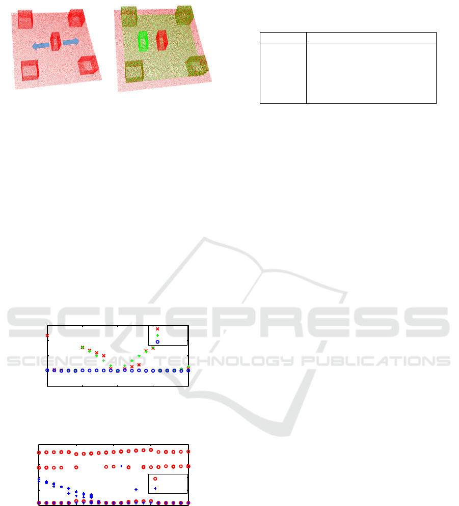
Figure 3: Inconsistency in simulated environment: left) re-

ference map (red), the central object is moved along axis

shown by arrows to introduce inconsistencies; right) the re-

ference map overlain with an inconsistent map (green).

central box being shifted along the x axis to produce

an inconsistency between the point clouds. The refe-

rence ground plane is extended for 2 meters to protect

against overlapping errors in the registration task. Fi-

gure 3 shows the simulated clouds: a) the reference

cloud with arrows showing the axis of the shift app-

plied to the central box; b) the same reference cloud

(red), an inconsistent input cloud (green) overlayed

on top. Finally an offset is applied to the input cloud

to misalign the point clouds for registration.

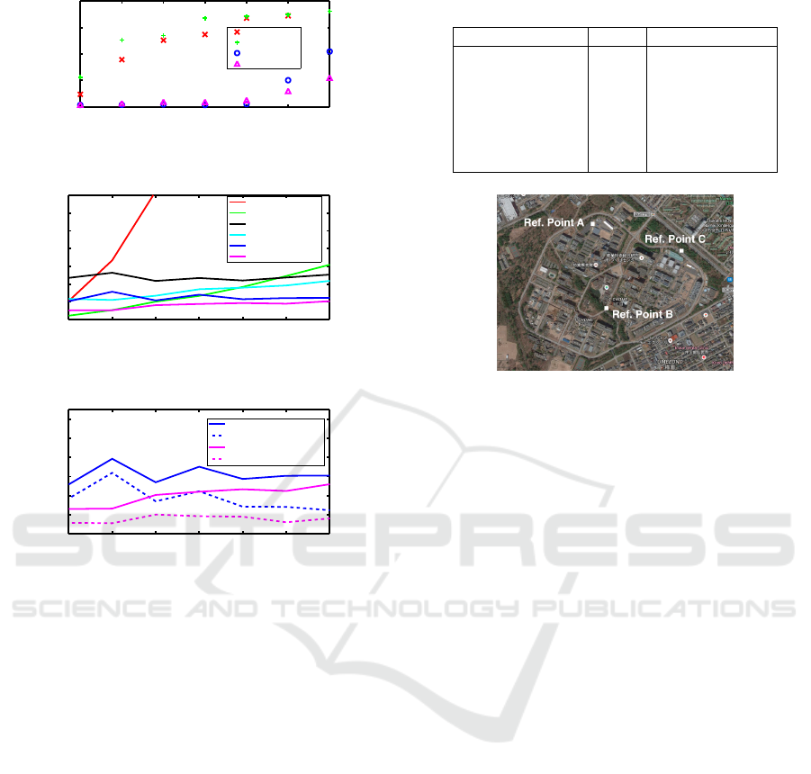
4.2 Registration with Inconsistencies

-1 -0.5 0 0.5 1

-0.05

0.05

0.1

Inconsistency X Offset (m)

Error (m)

ICP

PTP

LSPF

Average Registration Error with Inconsistency

-1 -0.5 0 0.5 1

0.5

1.5

Inconsistency X Offset (m)

Error (m)

IA-SAC

RANSAC

Registration Error with Inconsistency

Figure 4: Error in alignment transformation estimate versus

distance of point cloud inconsistency: a) average error for

LSPF, ICP and ICP-PTP methods; b) error for each trial of

RANSAC and IA-SAC methods.

For each trial, simulated reference and input point

clouds (10m × 10m) were generated with an inconsis-

tency x

of −1.0m to 1.0m along the x axis in steps of

0.1m being introduced to the central box. The entire

Table 1: Registration computation time for simulated incon-

sistent point clouds.

Method Ave. Comp. Time (S) (Parallel)

ICP 5.19

PTP 1.11

IA-SAC 23.19

RANSAC 62.75

LSPF 11.76 (5.05)

LSPF-A 8.07 (3.60)

input cloud was further offset by 1.0m on the same

axis for misalignment. Experiments were run on ma-

chine with an Intel Quad Core i7 64 bit processor.

LSPF detection was applied to the reference cloud

and a LSPF set generated. Then, LSPF, ICP, ICP-PTP,

RANSAC and IA-SAC registration methods were ap-

plied to the misaligned cloud sets, and the estimated

transformation and computation time of each method

was recorded. For each value of x

10 trials were per-

formed. Figure 4 shows the translational error of the

estimated alignment transformation for each value of

. Figure 4 a) shows the average translational error

for each x

over the 10 trials for LSPF, ICP and ICP-

PTP methods. It can be seen that both ICP and ICP-

PTP methods have an error proportional to the size of

the inconsistency when −0.5 ≥ x

≤ 0.5. LSPF, ho-

wever does not suffer such a decrease in performance.

The plot of error in individual trials in Figure 4

b) shows that the response for RANSAC and IA-SAC

methods are multi-modal; that is the registration pro-

cess converges into different minima depending on

randomness within the methods. While IA-SAC does

sometimes converge on the true minima (as well as

two other distinct minima), the subsequent ICP alig-

nment still suffers the same error as ICP and ICP-

PTP as noted above. In comparison, while the RAN-

SAC error is bi-modal, one minima roughly conver-

ging onto the value x

, the other minima converges

onto the true alignment, avoiding the errors seen in

the ICP and PTP methods.

The average computation time for each method,

over all trials, is shown in Table 1. RANSAC and IA-

SAC methods are computationally heavy due to sam-

pling and feature detection respectively, while ICP-

PTP is the fastest. Computation time for total LSPF

and for LSPF alignment only are given. A parallel

version of LSPF was also developed and computa-

tion times given. One feature of LSPF registration

is the ease of parallel processing, as multiple feature

detection and subsequent alignment processes can run

simultaneously with little synchronisation required.

4.3 Registration with Large Maps

While LSPF is the most accurate, it was shown to

be computationally heavy in comparison to ICP-PTP.

ICINCO 2018 - 15th International Conference on Informatics in Control, Automation and Robotics

278

10 15 20 25 30 35 40

0.05

0.1

0.15

0.2

Map Size (m)

Error (m)

ICP

PTP

LSPF

LSPF-PTP

Average Registration Error vs Map Size

10 15 20 25 30 35 40

Map Size (m)

Time (s)

ICP

PTP

LSPF

LSPF-PTP

LSPF(P)

LSPF-PTP(P)

Average Computation Time vs Map Size

10 15 20 25 30 35 40

Map Size (m)

Time (s)

LSPF(P)

LSPF-Align(P)

LSPF-PTP(P)

LSPF-PTP-Align(P)

LSPF Total vs Alignment Computation Time

Figure 5: Registration performance for various map sizes:

a) Error in estimated transformations for each method, b)

Total computation time for each method as well as for paral-

lellised execution of LSPF based methods (P), and c) Total

and just alignment computation time for LSPF and LSPF-

PTP registration (parallel).

This is because of the cost of feature detection in

LSPF and the relatively slow convergence of the ICP

algorithm used to align each LSPF region. Because

point matching based registration of point clouds tend

to increase exponentially with the amount of points

in the clouds, it is expected feature based approach

such as LSPF will scale better with map size. Here we

compare registration accuracy and computation time

for LSPF, ICP, ICP-PTP and LSPF-PTP (LSPF regis-

tration using ICP-PTP to align each feature region) for

maps with increasing ground plane sizes. The map si-

zes used and their approximate point cloud size are

given in Table 2.

Figure 5 a) shows the translational error of each

method for map sizes between 10m × 10m and 40m×

40m. The error for ICP and PTP increases linearly

with respect to map size. LSPF and LSPF-PTP er-

ror remains approximately 1/10

of ICP error, until

Table 2: Map size and approximate point cloud size. Label

column shows how map size is denoted in ﬁgures.

Map Size (m×m) Label Point Cloud Size

10 × 10 10 59,000

15 × 15 15 125,000

20 × 20 20 213,000

25 × 25 25 325,000

30 × 30 30 463,000

35 × 35 35 622,000

40 × 40 40 806,000

Figure 6: Places of overlap between captured MMS and

LCSM maps.

map size 35 when they start to increase, but are still

much lower than other methods (LSPF-PTP is less

than 1/3

the error at map size 40).

Figure 5 b) shows the average computation time of

LSPF, LSPF-PTP (and parallel versions of the two),

ICP and ICP-PTP methods for various map sizes. ICP

computation time increases exponentially and rapidly

rises out of view of the plot. LSPF and LSPF-PTP

computation time remains steady even for larger map

sizes. ICP-PTP computation starts of low but rises

gradually as map size increases, passing both LSPF

and LSPF-PTP. Parallel computation times for LSPF-

PTP are about one third ICP-PTP by map size 40.

Figure 5 c) shows LSPF total and alignment compu-

tation times. Alignment time remains less than one

quarter of total time for all map sizes.

5 REAL WORLD RESULTS

In this section we present registration results when ap-

plying LSPFs to real world point cloud data and com-

pare the performance with that of point-to-plane ICP

registration.

5.1 Real World Environment

A large 3D point cloud map of the AIST Tsukuba

Central Campus was constructed using a MMS map-

ping system. A low cost sensor based mapping sy-

stem (Yokozuka et al., 2015) captured paths within

the same environment, but months apart in time, ha-

Registration of Inconsistent Point Cloud Maps with Large Scale Persistent Features

279

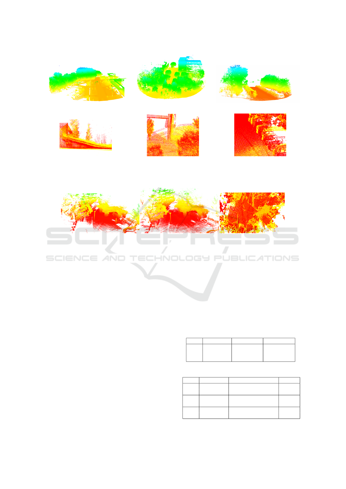
a) b) c)

d) e) f)

Figure 7: Real world experiment: MMS point clouds for place a) A, b) B and c) C. Inconsistencies between MMS (red) and

LCSM (yellow) point clouds: d) vegetation change in place A, e) inconsistent building surfaces in LCSM map in place B, f)

parked cars and leafy trees in place C.

a) b) c)

Figure 8: LSPF registration of ASL data sets: a) gazebo in summer, and b) winter, c) the aligned clouds from below.

ving some overlap with the MMS map at three places

(see Figure 6). MMS point clouds are accurate and

very dense. Here they have been subsampled down to

0.1m, but still remain approximately double the den-

sity than that of the Low Cost Sensor Map (LCSM)

clouds. Point clouds taken from the maps at the three

reference places are different in environment structure

and each have inconsistencies between the MMS and

LCSM data (see Figure 7):

• Place A: large open area with car park, vegetation

and buildings. Vegetation growth and parked cars

provide inconsistencies between clouds.

• Place B: Narrower road, with large buildings

and many leafy trees. Internal inconsistencies in

LCSM on building faces and ground plane.

• Place C: Narrow road area wisth large leafy trees

and parked cars, minimal structured buildings.

Given the structure of the environment it would be

expected that registration using LSPF would be most

helpful at place A. Indeed, given the structural incon-

sistencies in buildings in place B, and paucity of per-

sistent built structures in C, we would expect a degra-

dation of performance from A to C.

5.2 Real World Registration

Table 3 shows the map and point cloud sizes for the

MMS (reference) and LCSM (input) maps at each of

the locations. LSPF detection was performed on the

MMS clouds and then LSPF registration was used to

align input clouds. Table 4 presents the estimated

error in registration for map locations A, B and C,

as well as the computation time (total, detection and

Table 3: Real world MMS (Ref.) and LCSM (Input) map

and point cloud size.

Map Radius(m) Ref. Cloud. Input Cloud

A 50 1,812,000 1,016,000

B 50 4,447,000 4,442,000

C 25 619,000 194,000

Table 4: Real world MMS and LCSM registration results.

Map Method Time(s)[Det., Align] Err(m)

A PTP-ICP 113.73 0.1424

LSPF-PTP 50.71 [45.55, 5.16] 0.0308

B PTP-ICP 207.47 0.1504

LSPF-PTP 55.99 [46.98, 9.01] 0.0336

C PTP-ICP 13.86 0.1201

LSPF-PTP 21.73 [18.45, 3.28] 0.7575

ICINCO 2018 - 15th International Conference on Informatics in Control, Automation and Robotics

280

alignment). For comparison, results using ICP-PTP,

the best of the alternative methods in the simulation

results, are also presented. Ground truth is assigned

by manually aligning point clouds so reported error

should be treated with some caution.

Registration in places A and B using LSPFs was

both more accurate and required less computation

time than PTP-ICP. The presence of structured buil-

dings allows for LSPF based registration to overcome

the inconsistencies within the point clouds. The large

amount of vegetation however, causes the LSPF de-

tection time to increase, as more features are nee-

ded to successfully sample the unstructured elements

of the point clouds. Alignment time however is

very quick, approximately 5% that of PTP-ICP. Note,

LSPF times are using parallel computation.

Registration using LSPF in place C, however, fails

to converge on the correct transform. The lack of

structured buildings and the large amount of inconsis-

tencies (trees, parked cars), makes it difﬁcult to ﬁnd

features with a consistent registration transform.

5.3 Registration of an Open Data Set

Although many data sets are available to test registra-

tion algorithms, they typically consist of data scans

captured by moving a vehicle through an environ-

ment. ASL (Pomerleau et al., 2012) publish a data

set that contains point clouds built from scans captu-

red at different times of the year. The point cloud is of

a gazebo covered with vines and surrounding by large

trees. The authours describes this as a semi-structured

environment with seasonal changes. Example images

from a) summer and b) winter point clouds are shown

in Figure 8. The initial misalignment between the two

point clouds is approximately 1m.

Here we apply LSPF registration to align the sum-

mer and winter data sets. Although no ground truth

exists to quantitatively evaluate the alignment, Fi-

gure 8 c) shows the aligned clouds from below, where

it can be seen that the structured areas of the point

clouds such as the corners of the gazebo and the ed-

ges of the paths are closely aligned.

6 CONCLUSIONS

This paper presented a method for registration of

large scale inconsistent point cloud maps using Large

Scale Persistent Features. Feature detection was de-

tailed and a measure for evaluating features for re-

gistration based on number and orthogonality of nor-

mal density clusters was proposed. Simulated point

clouds of structured environments with inconsistent

regions were constructed to evaluate registration per-

formance. LSPF registration performance on simu-

lated point clouds was more accurate and faster than

other registration techniques for larger point cloud si-

zes. Real world MMS and LCS maps were merged,

with LSPF registration performing better for struc-

tured enivironments containing inconsistencies than

ICP point-to-plane, although the reverse was true for

unstructured environments. This result was expected

as LSPFs are speciﬁcally designed to detect large

structured regions that persist spatially and tempo-

rally. LSPF detection time also grows in unstructured

environments, as more samples are needed to cover

the distribution of unstructured point clouds.

Future work is to apply LSPF to a larger data set

of point clouds. Existing data sets tend to have point

cloud data captured from spatially and temporally

proximal locations, or are limited in extent such as

the ASL data set, so a large scale data set with signi-

ﬁcant inconsistencies between point clouds should be

constructed. Also, the LSPF detection process shoud

be optimised for speed as for large point clouds de-

tection computation time far exceeds alignment time.

Finally, the winner take all consensus sampling within

the set of LSPF estimated transforms can lead to in-

correct registration in unstructured environments. An

approach aggregating a number of transforms might

alleviate this problem.

REFERENCES

Besl, P. and McKay, N. (1992). A method for registration of

3-d shapes. In IEEE Transactions on Pattern Analysis

and Machine Intelligence, Vol. 15, No. 2.

Chen, Y. and Medioni, G. (1991). Object modeling by re-

gistration of multiple range images. In IEEE Interna-

tional Conference on Robotics and Automation.

Chetverikov, D., Svirko, D., and Stepanov, D. (2002). The

trimmed iterative closest point algorithm. In Interna-

tional Conference on Pattern Recognition.

Gelfand, N., Ikemoto, L., Rusinkiewicz, S., and Levoy, M.

(2003). Geometrically stable sampling for the icp al-

gorithm. In International Conference on 3D Digital

Imagine and Modeling.

Harris, C. and Stephens, M. (1988). A combined corner and

edge detector. In Fourth Alvey Vision Conference.

Holz, D., Ichim, A., Tombari, F., Rusu, R., and Behnke,

S. (2015). Registration with the point cloud library:

A modular framework for aligning in 3-d. In IEEE

Robotics and Automation Magazine, Vol. 22.

Lu, F. and Milios, E. (1997). Globally consistent range scan

alignment for environment mapping. In Journal Of

Autonomous Robots, Vol. 4.

Pomerleau, F., Liu, M., Colas, F., and Siegwart, R. (2012).

Challenging data sets for point cloud registration algo-

Registration of Inconsistent Point Cloud Maps with Large Scale Persistent Features

281

rithms. In International Journal of Robotic Research,

Vol. 31, No. 14.

Pyvanainen, T., Berclaz, J., Korah, T., Hedau, V., Aanja-

neya, M., and Grzeszczuk, R. (2012). 3d city mo-

deling from street level data for augmented reality ap-

plications. In In Proceedings of the International Con-

ference on 3D Imaging, Modeling Processing, Visua-

lization and Transmission.

Rusu, R. B., Blodow, N., and Beetz, M. (2009). Fast point

feature histograms (fpfh) for 3d registration. In IEEE

International Conference on Robotics and Automa-

tion.

Rusu, R. B. and Cousins, S. (2011). D is here: Point cloud

library (pcl). In IEEE International Conference on

Robotics and Automation.

Segal, A. V., Haehnel, D., and Thrun, S. (2009).

Generalized-icp. In Robotics: Science and Systems.

Shiratori, T., Berclaz, J., Harville, M., Shah, C., Li, T., Mat-

sushita, Y., and Shiller, S. (2015). Efﬁcient large-scale

point cloud registration using loop closures. In Inter-

national Conference on 3D Vision.

Tao, C. V. and Li, J. (2007). Advances in Mobile Mapping

Technology. Taylor & Francis Group.

Thompson, S., Yokozuka, M., Hashimoto, N., and Matsu-

moto, O. (2016). Registration of low cost maps within

large scale mms maps. In IEEE International Confe-

rence on Smart City.

Weber, C., Hahmann, S., and Hagen, H. (2010). Sharp fea-

ture detection in point clouds. In IEEE International

Conference on Shape Modeling and Applications.

Yokozuka, M., Hashimoto, N., and Matsumoto, O. (2015).

Low cost 3d mobile mapping system by 6dof locali-

zation using embedded sensors. In International Con-

ference on Vehicular Electronics and Safety.

ICINCO 2018 - 15th International Conference on Informatics in Control, Automation and Robotics

282