Singularity Loci and Kinematic Induced Constraints for an XY-Theta
Platform Designed for High Precision Positioning
Anas Hijazi, Jean-Franc¸ois Brethe and Dimitri Lefebvre
Groupe de Recherche en Electrotechnique et Automatique du Havre (GREAH),
Le Havre University, BP540, 76058 Le Havre, France
Keywords:
Singularity Analysis, Singular Surfaces, Jacobian Matrix, Redundant Manipulator Arm, XY-Theta Platform,
Design and Kinematics.
Abstract:
In this paper, the singularity analysis of an XY-Theta platform held by a serial redundant manipulator will be
illustrated in details. This XY-Theta platform has a patented kinematics designed to keep the final position
error below to 2 µm in its 300mm ×300mm workspace (Hijazi et al., 2015). These high performances are
obtained due to the combination of three factors: proximity to a singular configuration allowed by a specific
choice of the arm lengths to reduce the lever arm lengths, redundant kinematic chain to enlarge the dexterous
workspace and a two-step control using mechanical breaks set up on the furthest joints and exteroceptive
sensors in the final step. However, if the proximity of singularities is useful for the precision performance,
it may also cause some control problems. Consequently, it is crucial to identify the singularity loci and the
kinematic constraints they induce. This analysis is done in two cases: when the first joint is considered locked
and the robot is not redundant anymore and when the robot can be controlled using the four joints. In the
non-redundant case, the usual singularity surface degenerates into an helix. In the redundant case, singularity
surfaces may appear in specific configurations. In both cases, the induced kinematic constraints are analyzed
and strategies are proposed to overcome the problems.
1 INTRODUCTION
It is highly recommended to identify the singulari-
ties of a manipulator during the design stage, in order
to be able to take into account their location for the
control of the robot. Indeed, near singular configu-
ration, the robot control algorithms may lead to large
joint velocities or encounter instantaneous loss of dof
(degree of freedom) (Merlet, 2006). This singularity
analysis has been performed by many researchers on
several different robots (Wenger, 2007),(Chablat and
Wenger, 1998).
A robot has n dof in the operational space descri-
bed by x = (x
1
,...,x
n
) and m degrees of mobility in
the actuator space described by q = (q
1
,...,q
m
). For
serial robots, actuator and operational coordinates are
linked by the forward kinematic function x = f (q).
The Jacobian matrix appears after differentiating this
relation: dx = Jdq. Mathematically, considering the
case of non-redundant serial robots, a loss of one or
more dof is characterized by a drop in the rank of the
Jacobian, implying det(J) = 0. If the serial robot is
redundant, the location of the singularities are found
using the following formula: det(J ×J
T
) = 0 (Khalil
and Dombre, 2002), (Tsai, 1999).
For parallel robots, the closed-form kinematic
equations link the actuator and operational coordina-
tes: g(x,q) = 0 and two matrices A and B appear af-
ter differentiation:A(x,q)dx+B(x,q)dq = 0. In (Gos-
selin and Angeles, 1990), Gosselin defined the serial
and parallel singularities and proposed a classification
of singularities into three types depending on the to-
pology of the robot and the impact on the control:
1. Singularities of type I occur at the workspace
boundaries and can be avoided by motion plan-
ning. This type named inverse kinematic singula-
rity can be found in serial det(J) = 0 or parallel
det(B) = 0 manipulators.
2. Singularities of type II result in additional dof at
the end-effector and the mechanism cannot main-
tain its static equilibrium upon external forces.
This type named direct kinematic singularity is
specific to parallel manipulators.
3. Singularities of type III appear where both singu-
larities of type I and II are present. Consequently
Hijazi, A., Brethe, J-F. and Lefebvre, D.
Singularity Loci and Kinematic Induced Constraints for an XY-Theta Platform Designed for High Precision Positioning.
DOI: 10.5220/0006827700390048
In Proceedings of the 15th International Conference on Informatics in Control, Automation and Robotics (ICINCO 2018) - Volume 2, pages 39-48
ISBN: 978-989-758-321-6
Copyright © 2018 by SCITEPRESS – Science and Technology Publications, Lda. All rights reserved
39

this type is also specific to parallel manipulators.
In (Merlet, 1989), Merlet proposed a new method
based on Grassmann line-geometry to detect the sin-
gularities. Zlatanov thought that the role played by
passive joint velocities was not utterly taken into ac-
count, and analyzed the problem in a more general
way in (Zlatanov et al., 1995). He introduced the for-
ward (FIKP) or the inverse (IIKP) instantaneous ki-
nematic problems, interpreting singularities as a lo-
cus where the previous problems were undetermined.
If the definitions of singularities seem now to cover a
large spectrum of robot topology, it is still difficult
to identify them. In some simple cases, analytical
solutions can be found, but most of the time, nume-
rical methods must be developed. For instance, in
(Bohigasa et al., 2013) a numerical computation of
manipulator singularities is presented. More research
was realized by Malek to study the singularities in the
presence of joint limits, concerning non-redundant ro-
bots (Abdel-Malek and Yeh, 2000) or even redundant
robots (Mi et al., 2011).
In this paper, we study the singularity loci of
an XY-Theta platform developed in our laboratory
GREAH, designed to reduce the final position error
below to 2 µm (Breth
´
e, 2011b), (Hijazi et al., 2014),
(Breth
´
e et al., 2013). Our motivations to analyze the
singularity loci of this platform are:
1. To know these undesirable postures of the singula-
rity that should be recognized and avoided during
the design, planning and control.
2. To operate the robot close to them to obtain a fine-
positioning (Kao et al., 2007). In (Breth
´
e, 2011a),
it is shown that the spatial resolution and repea-
tability of a 2R plane serial robot is much better
close to the center of the workspace, ie close to a
singularity. The explanation is that the lever arm
is short when the point lies near the singularity.
In section 2, the XY-Theta platform is presented in
details. In section 3, the Jacobian matrix of the plat-
form is calculated and the singularity configurations
are analyzed. Then the singularity surfaces are drawn
in the non-redundant and redundant cases. Finally, the
conclusions are presented in section 4.
2 XY-Theta PLATFORM AND THE
ROBOT PRECISION
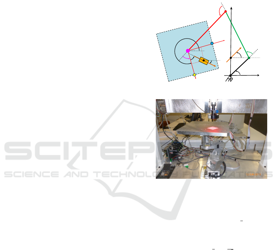
2.1 Overview of the Platform Structure
The XY-Theta platform consists of a 300mm ×
300mm square and is held by a redundant kinematic
chain of four motorized vertical revolute joints, with
respective angles θ
1
, θ
2
, θ
3
and θ
4
displayed in Fig. 1.
The first arm length is L
1
= 30 mm. The second and
the third arm lengths are L
2
= L
3
= 120 mm. The
prototype is displayed in Fig. 2.
Y
1
Y
2
O
3
θ
3
Y
L
2
L
3
a
X
1
X
2
O
1
O
2
O
4
θ
1
θ
2
θ
4
A
X
Y
P
I
L
1
a
Ω
ψ
ψ
0
P=(X,Y)
Figure 1: Diagram of the XY-Theta platform kinematics.
Figure 2: Micro positioning platform: general view.
This robot is designed to achieve precise positio-
ning in the vicinity of a specific point named P
I
”point
of interest” in the workspace. O
1
P
I
O
2
is an isosce-
les, right-angled triangle when θ
1
=
π
4
. The choice
of this value is because the lever arm lengths between
the first axis O
1
and the second axis O
2
from P
I
are
then minimum. These lengths can be calculated as:
O
1
P
I
= O
2
P
I
= L
1
×cos(
π
4
) =
30
√
2
= 21.21mm and
there are 6 times shorter than the second or third arm
lengths of 120 mm. Moreover, the micro-movements
induced by a micro-rotation of θ
1
and θ
2
are orthogo-
nal.
There is an additional motorized vertical prisma-
tic axis, which can hold a tool, for instance a grip-
per to grasp a workpiece. The vertical axis projection
on the base lies at P
I
. The robot is designed so that
any workpiece on the platform can be picked and pla-
ced somewhere else on the platform with the desired
orientation. Thus the operational space enables three
degrees of freedom for the workpiece. To characterize
the dof of the workpiece, the operational coordinates
ICINCO 2018 - 15th International Conference on Informatics in Control, Automation and Robotics
40

x = (X,Y, Ω) of the workpiece are given in the plat-
form frame (O
4
X
2
Y
2
). (O
1
X
1
Y
1
) is the world frame
coordinate system.
Let A be the rotation angle of the platform relative
to the world frame:
A = θ
1
+ θ
2
+ θ
3
+ θ
4
(1)
Let Ψ be the the rotation angle of the workpiece
relative to the world frame:
Ψ = A + Ω (2)
The gripper fixed on the vertical axis can grasp
a workpiece when the workpiece center P lies at P
I
with the specific orientation Ψ
0
, sketched by the green
arrow. Then we have necessarily: A +Ω = Ψ
0
⇒A =
−Ω + Ψ
0
.
2.2 The Coarse and Fine Positioning
Modes
The platform can be operated in two different modes:
• The coarse positioning mode uses the four axes.
In this case, the expected repeatability is in the
range of 5-10 micrometers, which is equivalent to
high quality industrial SCARA of the same reach.
• The fine positioning mode consists of two steps.
In the first step, the workpiece is moved below the
vertical axis at point P
I
with the desired orienta-
tion using the four axes and θ
1
is set to
π
4
. Then,
in the second step, the 3rd and 4th axes are bloc-
ked using mechanical brakes set up on these axes
and the positioning error can then be reduced mo-
ving only the first and second axes. The choice of
the blocked and moving axes depends on the lever
arm length and from inception, the mechanism is
designed to optimize the link lengths to reduce the
final error. All points of the platform workspace
can benefit from the high precision performance
(Breth
´
e et al., 2013),(Hijazi et al., 2014).
2.3 Kinematics Modeling
2.3.1 Forward Kinematics Function
The world [W L] and platform [PT ] coordinates frames
are here considered. The forward kinematics function
links the actuator coordinates θ = (θ
1
,θ
2
,θ
3
,θ
4
)
T
with the operational coordinates x = (X,Y, Ω)
T
. The
equations are the following:
−−→
O
1
P =
−−→
O
1
P
I
=
−−−→
O
1
O
4
+
−−→
O
4
P
I
(3)
−−−→
O
1
O
4
[W L]
=


L
1
.cos(θ
1
) + L
2
.cos(θ
1
+ θ
2
)+
(1)
L
3
L
1
.sin(θ
1
) + L
2
.sin(θ
1
+ θ
2
)+
(2)
L
3


(4)
Where
(1)
L
3
= L
3
.cos(θ
1
+ θ
2
+ θ
3
) and
(2)
L
3
= L
3
.sin(θ
1
+ θ
2
+ θ
3
). This matrix introdu-
ced in equation 4 will be named as: B (θ
1
,θ
2
,θ
3
).
−−→
O
4
P
I
[PT ]
=

X
Y

(5)
−−→
O
4
P
I
[W L]
=

cos(A) −sin(A)
sin(A) cos(A)

×

X
Y

[PT ]
(6)
The matrix:

cos(A) −sin(A)
sin(A) cos(A)

will be named
as R(A).
Ω = Ψ
0
−A (7)
Once the four angles (θ
1
,θ
2
,θ
3
,θ
4
) are given, the re-
solution of the equations leads to a unique solution.
2.3.2 Inverse Kinematic Modeling
The inverse kinematics model is used to calculate the
joint coordinates θ in terms of the operational coordi-
nates x. The robot being redundant, there is an infinity
of solutions.
Let us study the inverse kinematic function when
θ
1
is set to π/4, so that the robot is not redundant
anymore.
The coordinates of the point of interest P
I
are:
P
I
=

0
L
1
×sin(θ
1
)

=

0
L
1
/
√
2

(8)
The coordinates of O
4
can first be computed using
the known angle A = Ψ
0
−Ω.
O
4
= P
I
+ R(A) ×

X
Y

(9)
The coordinates of O
2
can easily be calculated as
θ
1
= π/4. Then θ
2
and θ
3
are the solutions of a usual
geometric problem, consisting of connecting O
2
and
O
4
with two links and two rotoid joints (inverse kine-
matics function of a 2R planar serial robot).
At this stage, θ
1
,θ
2
and θ
3
are known and the de-
sired orientation of the platform Ω is also known, so
θ
4
can be deduced:
θ
4
= Ψ
0
−Ω −θ
1
−θ
2
−θ
3
(10)
We set now Ψ
0
= 0 so Ω = −(θ
1
+ θ
2
+ θ
3
+ θ
4
).
Singularity Loci and Kinematic Induced Constraints for an XY-Theta Platform Designed for High Precision Positioning
41

3 SINGULARITY ANALYSIS
In this section, singularity analysis of the XY-Theta is
performed, based on the Jacobian of the manipulator.
In our case, a serial robot is studied, so a singularity
of the first type presented by Gosselin (Gosselin and
Angeles, 1990) will be expected. XY-Theta platform
is a kinematic chain consisting of a set of rigid bo-
dies connected to each other with joints. This chain
is also characterized by a set of inputs corresponding
to the 4-dimensional vector θ = (θ
1
, θ
2
,θ
3
,θ
4
) of the
actuated joints, and by a set of output coordinates cor-
responding to an 3-dimensional vector x = (X,Y, Ω).
The relation between the input and output coordinates
is:
x = f (θ) (11)
3.1 Jacobian Matrix
By differentiating Eq. 11 with respect to time and de-
fining the Jacobian matrix as J = d f /dθ the following
equation is obtained:
˙
x = J(θ) ×
˙
θ (12)
Eq. 3 and 8 lead to Eq. 13.

0
L
1
/
√
2

= B (θ
1
,θ
2
,θ
3
) + R(A) ×

X
Y

(13)
By solving Eq. 13, the coordinates (X,Y, Ω) are
obtained with Eq. 14 and 15.

X
Y

= R(A)
−1
×

0
L
1
/
√
2

−R(A)
−1
×B(θ
1
,θ
2
,θ
3
)
(14)
Ω = −A = −(θ
1
+ θ
2
+ θ
3
+ θ
4
) (15)
Therefore in the general case, the Jacobian matrix
will be composed of four columns:
J =
h
~
J
1
~
J
2
~
J
3
~
J
4
i
(16)
3.1.1 Non-redundant Case
Here, θ
1
is set to π/4 as presented in section 2 so the
robot is not redundant. In this case the Jacobian is
given by:


˙
X
˙
Y
˙
Ω


=
(1)
J(θ) .


˙
θ
2
˙
θ
3
˙
θ
4


(17)
(1)
J(θ)=



∂
∂θ
2
(X)
∂
∂θ
3
(X)
∂
∂θ
4
(X)
∂
∂θ
2
(Y )
∂
∂θ
3
(Y )
∂
∂θ
4
(Y )
∂
∂θ
2
(Ω)
∂
∂θ
3
(Ω)
∂
∂θ
4
(Ω)



=
h
~
J
2
~
J
3
~
J
4
i
(18)
3.1.2 Redundant Case
Here, the four arms of the robot are free to move. In
this case the Jacobian is given by:


˙
X
˙
Y
˙
Ω


=
(2)
J(θ) .




˙
θ
1
˙
θ
2
˙
θ
3
˙
θ
4




(19)
(2)
J(θ)=



∂
∂θ
1
(X)
∂
∂θ
2
(X)
∂
∂θ
3
(X)
∂
∂θ
4
(X)
∂
∂θ
1
(Y )
∂
∂θ
2
(Y )
∂
∂θ
3
(Y )
∂
∂θ
4
(Y )
∂
∂θ
1
(Ω)
∂
∂θ
2
(Ω)
∂
∂θ
3
(Ω)
∂
∂θ
4
(Ω)



(20)
3.2 Singular Surfaces
3.2.1 Non-redundant Case
In this case, the serial manipulator presents singulari-
ties of type I named boundary or interior singularities
(Tsai, 1999),(Khalil and Dombre, 2002). Boundary
singularities appear when the manipulator is fully
stretched out, interior singularities when the manipu-
lator is folded back on itself. The boundary and in-
terior singularities can therefore be determined from
the analytical expression of the determinant:
det(
(1)
J(θ)) = 0 (21)
The solutions of this equation are: S
1
=
{
θ
3
= 0
}
,
S
2
=
{
θ
3
= ±π
}
.
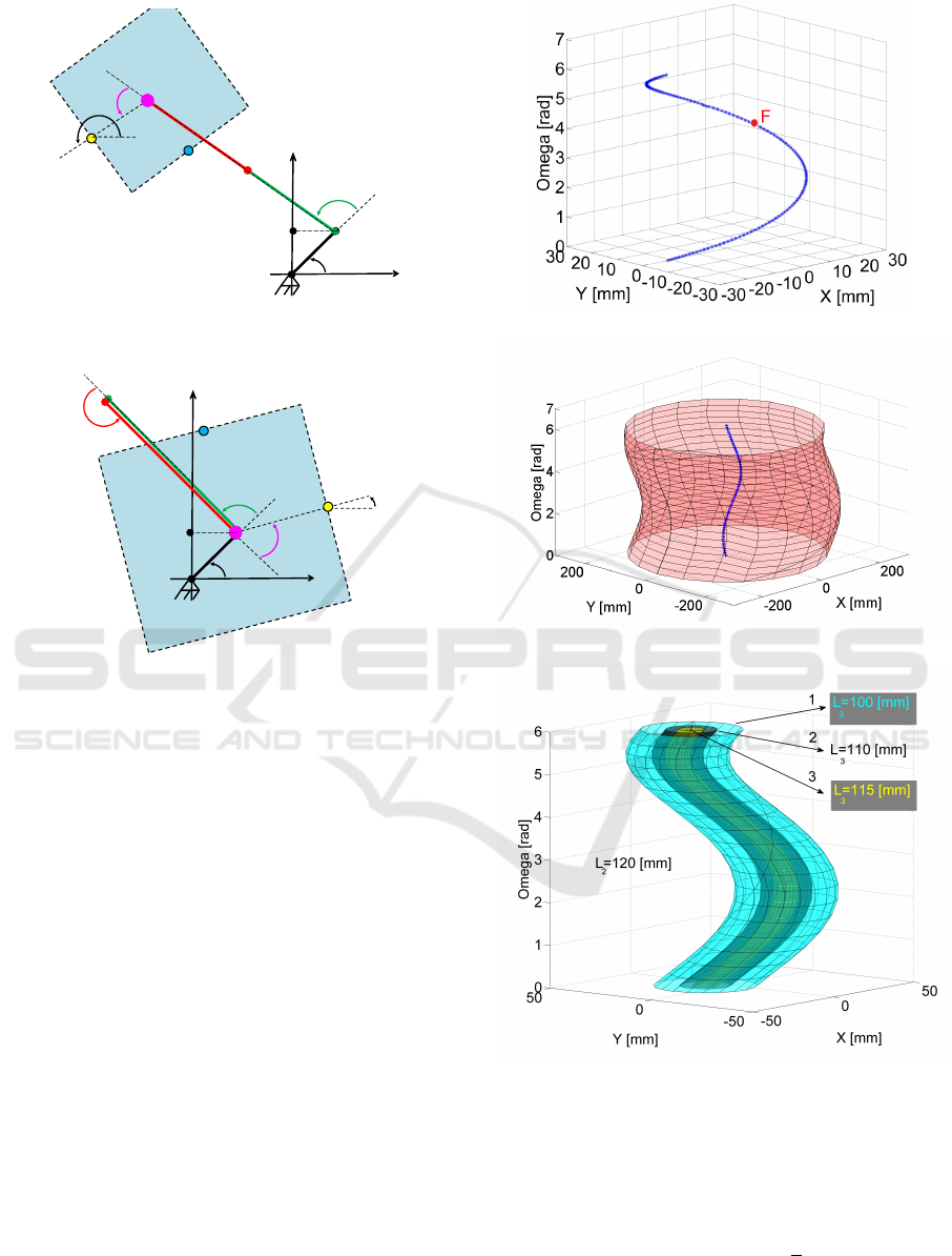
The singular configuration S
1
is displayed in Fig. 3
when the third arm L
3
is fully stretched out and se-
cond one S
2
is displayed in Fig. 4 when the third arm
L
3
is folded back on itself.
Let us draw the boundary singularity surface when
θ
3
= 0. The conditions are the following: θ
1
= π/4,
−π ≤ θ
2
≤ π , −π ≤ θ
4
≤ π. The singularity sur-
face in red is displayed in Fig. 6. Let us draw the
interior singularity surface in blue when θ
3
= π. The
conditions are the following: θ
3
= π, −π ≤ θ
2
≤ π
and −π ≤ θ
4
≤ π. The singularity surface is also dis-
played in Fig. 5 and Fig. 6.
In this particular case, the singularity locus is not
a surface anymore but it is an helix of radius O
4
P
I
=
L
1
×cos(
π
4
) =
30
√
2
= 21.21mm and pitch 2π. This case
ICINCO 2018 - 15th International Conference on Informatics in Control, Automation and Robotics
42

Y
1
O
O
4
θ
4
L
3
A
X
1
Y
1
O
1
O
2
O
3
θ
1
θ
2
θ
3
=0
L
1
L
2
P
I
Figure 3: Singularity configurations corresponding to S
1
when θ
3
= 0.
Y
1
O
3
θ
2
θ
3
=π
L
2
L
3
A
X
1
O
1
O
2
O
4
θ
1
θ
4
L
1
P
I
Figure 4: Singularity configurations corresponding to S
2
when θ
3
= π.
is unusual and it is worth explaining its origin and the
specific kinematic problems linked to this.
Usually in a 3D output space, the singularity locus
is a surface. Here it is only a line. This phenomenon
occurs because the lengths of the 2nd and 3rd arm are
identical L
2
= L
3
= 120[mm]. If these lengths were
different, the singularity locus would be a surface
delineating an helicoidal cylinder. The end-effector
(EE) could not go in the interior of this helicoidal
cylinder because it would be outside the workspace.
This is clearly illustrated in Fig. 7 where the helicoi-
dal cylinders are drawn for different lengths of L
3
, L
2
being constant at 120[mm].
The radius of the cylinder section in the XY plane
is equal to
|
L
3
−L
2
|
. When L
2
= L
3
the helicoidal cy-
linder degenerates into an helix. The underlying que-
stion is then the following: as the volume of this helix
is nil, can we consider that the workspace is plain? In
fact, this is the case because the EE can be anywhere,
but when the EE lies on the helix locus, some control
problems occur which will be now described in detail.
First, let us prove that
~
J
2
is always tangent to the
helix. For this, let us consider that the platform is
stationary as detailed in Fig. 8.
The mechanism has then four actuated revolute
Figure 5: Singularity curve when θ
3
= π.
Figure 6: Singularity surface and singularity curve when the
robot is non-redundant.
Figure 7: Workspace evolution when L
2
and L
3
are diffe-
rent.
joints and the forward kinematics function can be ex-
pressed as:
X = L
3
cos(π −θ
4
) + L
2
cos(π −θ
4
−θ
3
) +C
Y = L
3
sin(π −θ
4
) + L
2
sin(π −θ
4
−θ
3
) + D
Ω = −θ
4
−θ
3
−θ
2
−θ
1
(22)
where L
0
= L
1
/
√
2, C =
L
1
cos(π −θ
4
−θ
3
−θ
2
) + X
x
, D =
L
1
sin(π −θ
4
−θ
3
−θ
2
) + Y
y
, X
x
=
Singularity Loci and Kinematic Induced Constraints for an XY-Theta Platform Designed for High Precision Positioning
43

X
1
Y
1
O
1
O
-θ
1
-π/2
-θ
2
Y
P
I
L
1
Ω
L
0
O
2
O
3
O
4
-θ
3
π-θ
4
X
L
2
L
3
Figure 8: kinematics of the planar robot considering the
platform stationary.
L
0
cos(π −θ
4
−θ
3
−θ
2
−θ
1
−π/2) and
Y
y
= L
0
sin(π −θ
4
−θ
3
−θ
2
−θ
1
−π/2).
The locus of singularity corresponds to θ
1
= π/4
and θ
3
= π. As L
2
= L
3
, after simplification, the equa-
tions are the following:
s =


X = L
0
cos(θ
4
+ θ
2
+ π/4)
Y = −L
0
sin(θ
4
+ θ
2
+ π/4)
Ω = −θ
4
−θ
3
−θ
2
−θ
1


(23)
We recognize here the equations of an helix which
can be parametrized with a = θ
2
+ θ
4
. The tangent
vector to the helix is obtained by differentiating the
previous equation and leads to the vector t = ∂s/∂a:
t =


−L
0
sin(a + π/4)
L
0
sin(a −π/4)
−1


(24)
On the other hand, after differentiating the for-
ward kinematic function expressed in Eq. 22 with re-
spect to θ
2
, the expression of
~
J
2
is obtained:
~
J
2
=


L
0
sin(π/2 −θ
1
−θ
2
−θ
3
−θ
4
) −G
L
1
cos(−θ
2
−θ
3
−θ
4
) −H
−1


(25)
Where G = L
1
sin(−θ
2
−θ
3
−θ
4
) and H =
L
0
cos(π/2 −θ
1
−θ
2
−θ
3
−θ
4
).
Then on the helix, setting θ
1
= π/4 and θ
3
= π,
the value of
~
J
2
is the following:
~
J
2
=


−L
0
sin(θ
2
+ θ
4
+ π/4)
L
0
sin(θ
2
+ θ
4
−π/4)
−1


(26)
It can be seen that t (a = θ
2
+ θ
4
) =
~
J
2
(θ
1
= π/4, θ
2
,θ
3
= π, θ
4
) and consequently
~
J
2
is tangent to the helix.
When L
2
= L
3
and θ
3
= π, the centers of axes
2 and 4 lie on the same point, thus the velocities
vectors
~
J
2
and
~
J
4
are identical. The velocity vector
~
J
3
is always different from
~
J
2
. For every point on
the helix, there is an infinity of solutions verifying
θ
2
+ θ
4
= constant.
For instance, let us consider the
point F on the helix corresponding to
{
θ
1
= π/4, θ
2
= −π/4, θ
3
= π, θ
4
= 0
}
. The
coordinates of F in the output space is
{
X = 21.21[mm],Y = 0[mm], Ω = π[rad]
}
. All
combinations θ
2
+ θ
4
= −π/4 will give the same
location O
4
P
I
= F as illustrated in Fig. 9.
X
Y
1
O
4
θ
4
L
P
I
θ
2
A
θ
2
X
1
O
1
O
2
O
3
θ
1
θ
3
=π
L
1
L
2
L
3
P
I
θ
2
Figure 9: Infinity of configuration corresponding to the
point F on the singularity helix.
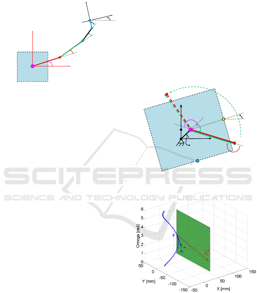
Figure 10: Instantaneous motion of the EE at point F when
θ
2
= −π/4.
In the location F, the expression of
~
J
2
is indepen-
dent of θ
2
or θ
4
. It is not the case of the expression
of
~
J
3
which depends explicitly of θ
2
or θ
4
. It can be
shown that
~
J
2
is always tangent to the helix, whereas
~
J
3
changes its size and direction depending on θ
2
.
For instance, when θ
2
= −π/4, the velocity vector
is necessarily in the plane Y Ω obtained by all linear
ICINCO 2018 - 15th International Conference on Informatics in Control, Automation and Robotics
44

combinations of
~
J
2
and
~
J
3
as displayed in Fig. 10. It
is impossible to move in directions that would not be
enclosed in the Y Ω plane.
Now if θ
2
= π/4, the vectors
~
J
2
,
~
J
3
defined a dif-
ferent plane displayed in Fig. 11, which is not verti-
cal anymore. It is only possible to move in directions
enclosed in this plane. So theoretically, it is possi-
ble from this singular point F to move in every di-
rection but this is not always possible instantly. If
the desired direction is not enclosed in the plane re-
sulting from the combinations of
~
J
2
,
~
J
3
, the robot has
to maneuver and change the angles θ
2
and θ
4
keeping
θ
2
+ θ
4
= −π/4 so that the EE still lies at the point F
but the direction of
~
J
3
changes to be in the final desi-
red plane where the EE has to move.
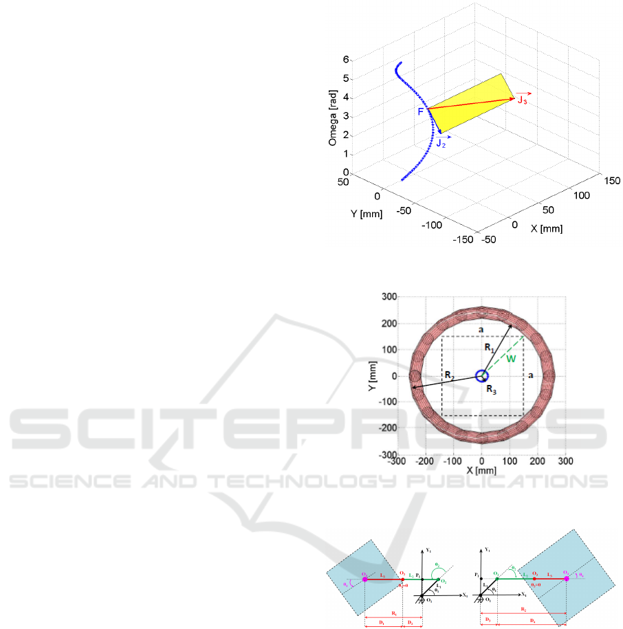
A projection of the singularity surface and curve
in the XY plane is presented in Fig. 12. The distance
R
3
= O
4
P
I
= 21.21 [mm] is already known. Fig. 13
displays the two configurations used to compute R
1
and R
2
, minimum and maximum radius of the pro-
jected surface. Results based on Fig. 13 are R
1
=
D
1
+ D
2
= L
2
+ L
3
−O
2
P
I
= 120 + 120 − 21.21 =
218.79[mm] and R
2
= D
4
+ D
3
= L
2
+ L
3
+ O
2
P
I
=
120 + 120 + 21.21 = 261.21 [mm]. It can be clearly
seen in Fig. 12 where the workspace of the platform
a × a = 300[mm] × 300 [mm] is projected, that the
workspace was designed to avoid the boundary sin-
gularities. But the helix singularity curve is definitely
inside the workspace and we have to take this into ac-
count.
3.2.2 Redundant Case
In the case of a redundant robot m > n, the Jacobian
matrix
(2)
J(θ) is not square. Singularities correspond
to det(
(2)
J(θ) ×
(2)
J(θ)
T
) = 0. This equation can be ex-
panded using the Cauchy-Binet formula introducing
the p = (n,m) minors Q
k
of maximum size extracted
from matrix J:
det(
(2)
J(θ) ×
(2)
J(θ)
T
) =
p
∑
k=1
(det(Q
k
)) ×(det(Q
T
k
))
(27)
=
∑
p
k=1
(det(Q
k
))
2
In our case: m = 4 and n = 3, and the equation
implies that the determinant of all minors is nil:
det(
(2)
J(θ) ×
(2)
J(θ)
T
) = 0 ⇒(∀k = 1 : 4),det(Q
k
) = 0
(28)
The solutions of these equations is a set of four
solutions:
Figure 11: Instantaneous motion of the EE at point F when
θ
2
= π/4.
Figure 12: A projection of the singularity surface and curve
in the XY plane in the non-redundant case.
Figure 13: The configuration corresponding of the mini-
mum radius R
1
in the left and the other one corresponding
of the maximum radius R
2
in the right.
1. S
3
=
{
θ
2
= 0, θ
3
= 0
}
: the second and third arms
are fully stretched out. The singularity surface
is obtained for −π ≤ θ
1
≤ π and −π ≤ θ
4
≤ π
and displayed in Fig. 14. This surface corre-
sponds to the boundary of the workspace. The
configuration of the platform for the point M
where
{
θ
1
= −1.88, θ
2
= 0, θ
3
= 0, θ
4
= −0.31
}
and belonging to this singularity surface is also
displayed.
2. S
4
=
{
θ
2
= ±π, θ
3
= 0
}
: the second arm is fully
Singularity Loci and Kinematic Induced Constraints for an XY-Theta Platform Designed for High Precision Positioning
45

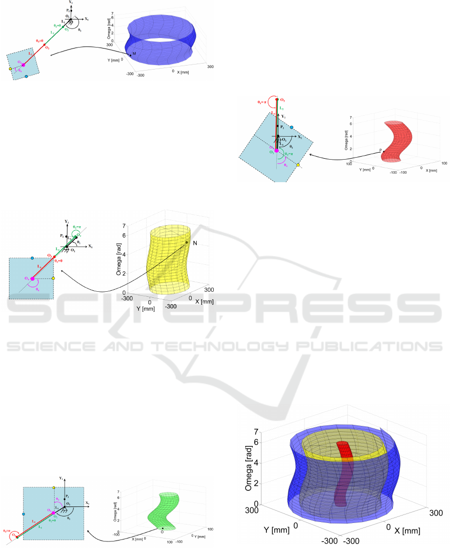
Figure 14: Singularity surface when S
3
=
{
θ
2
= 0,θ
3
= 0
}
.
folded back on itself and the third arm is fully
stretched out. The singularity surface is obtai-
ned for −π ≤ θ
1
≤ π and −π ≤ θ
4
≤ π and dis-
played in Fig. 15. This surface does not cor-
respond to the boundary of the workspace but
lies in the interior of the workspace. The con-
figuration of the platform for the point N where
{
θ
1
= 1.25, θ
2
= π, θ
3
= 0, θ
4
= 1.88
}
and belon-
ging to this singularity surface is also displayed.
Figure 15: Singularity surface when S
4
=
{
θ
2
= ±π,θ
3
= 0
}
.
3. S
5
=
{
θ
2
= 0, θ
3
= ±π
}
: the second arm is fully
stretched out and the third arm is fully folded
back on itself. The singularity surface is obtai-
ned for −π ≤ θ
1
≤ π and −π ≤ θ
4
≤ π and dis-
played in Fig. 16. This surface does not cor-
respond to the boundary of the workspace but
lies in the interior of the workspace. The con-
figuration of the platform for the point O where
{
θ
1
= −2.88, θ
2
= 0, θ
3
= π, θ
4
= 1.25
}
and be-
longing to this singularity surface is also dis-
played.
Figure 16: Singularity surface when S
5
=
{
θ
2
= 0,θ
3
= ±π
}
.
4. S
6
=
{
θ
2
= ±π, θ
3
= ±π
}
: the second arm is fully
folded back on itself and the third arm is also fully
folded back on itself. The singularity surface is
obtained for −π ≤ θ
1
≤ π and −π ≤ θ
4
≤ π and
displayed in Fig. 17. This surface does not corre-
spond to the boundary of the workspace but lies
in the interior of the workspace. The singula-
rity surface of case 3 and 4 are in fact identical.
The configuration of the platform for the point
P where
{
θ
1
= −1.57, θ
2
= π, θ
3
= π, θ
4
= 1.25
}
and belonging to this singularity surface is also
displayed.
Figure 17: Singularity surface when S
6
=
{
θ
2
= ±π,θ
3
= ±π
}
.
Let us analyze each of these cases and draw the
singularity surfaces which are displayed in Fig. 18.
Concerning S
3
, the second and third arms are fully
stretched out. The singularity surface in blue is obtai-
ned for −π ≤ θ
1
≤ π and −π ≤ θ
4
≤ π. Regarding
S
4
, the second arm is fully folded back on itself and
the third arm is fully stretched out. The singularity
surface in yellow is obtained for −π ≤ θ
1
≤ π and
−π ≤ θ
4
≤ π. Concerning S
5
, the second arm is fully
stretched out and the third arm is fully folded back on
itself. The singularity surface in red is obtained for
−π ≤ θ
1
≤ π and −π ≤ θ
4
≤ π. Versus S
6
, the se-
cond arm is fully folded back on itself and the third
arm is also fully folded back on itself. The singula-
rity surface are identical with former case S
5
in red
for −π ≤ θ
1
≤ π and −π ≤ θ
4
≤ π.
Figure 18: Singularity surfaces when the robot is redundant.
3.2.3 Discussion about the Kinematic Induced
Constraints
Considering the non-redundant case, the trajectory of
the robot EE can cross the singularity helix without
ICINCO 2018 - 15th International Conference on Informatics in Control, Automation and Robotics
46

causing any specific problem if the trajectory is dif-
ferentiable. Indeed, the tangent to the direction of
the arrival defines the velocity vector and this same
direction can be used to leave the singularity, be-
cause the velocity will necessarily be inside the tan-
gent plane defined by
~
J
2
and
~
J
3
. However the draw-
backs of singularity will always be present in the vi-
cinity of the singularity, if the trajectory followed by
the EE is close to the helix, then the velocity of the
joints would be important.
In the redundant case, the analysis is different.
The singularity surfaces can be avoided because in
this case, the inverse kinematic function leads to
an infinity of solutions for each point inside the
workspace. Because of redundancy, it is always pos-
sible to choose a set of input coordinates (θ
1
,..., θ
4
)
to avoid crossing a singular configuration. Of course,
this implies implementing this constraint in the cont-
rol loop, using the manipulability index for instance.
If following a given trajectory the robot has unfortu-
nately reached the singularity surface, the velocity is
then constrained to be in the plane tangent to the sin-
gularity surface, and the robot loses instantly one dof
in the (X,Y, Ω) space. This can cause great problems
and sometimes the EE would not be able to follow the
planned trajectory. Indeed let us study the case when
the trajectory crosses the singularity surface without
arriving in the tangent plane. If the control is well
done in the (θ
1
,..., θ
4
) space, the singular configura-
tions are avoided and in fact the singularity surface
does not exist. The robot EE can follow the trajectory
without any problem. If the control does not manage
to avoid the singularity, and a singular configuration
in the space (θ
1
,..., θ
4
) occurs just when the EE arrives
on the potential singularity surface in (X,Y, Ω). Then
necessarily, the EE has to leave the singular point with
a velocity vector in the plane tangent to this surface.
The robot will not be able to follow the initial trajec-
tory anymore.
4 CONCLUSION
In this paper, the singularity loci of an XY-Theta plat-
form held by a serial manipulator have been analy-
zed in details. The high precision performances of
the platform result from the proximity of singulari-
ties, but require to identify the loci and analyze the
kinematic problems that could occur. This analysis
is done in two steps: firstly, when the robot is non-
redundant, an unusual case is brought to light where
the surface singularity degenerates into an helix. This
singularity helix does not prevent the robot EE to fol-
low a differentiable trajectory, but some usual draw-
backs are encountered if the trajectory is close to the
helix. Secondly, the four joints are used to control
the robot and the potential singularity loci are identi-
fied. Here, if the control manages to avoid the singular
configurations in the (θ
1
,..., θ
4
) space, then the robot
can move inside the dexterous workspace without any
restrictions. Otherwise, if unfortunately, the singular
configuration in (θ
1
,..., θ
4
) space is encountered while
the EE lies on the singularity surfaces, then the robot
EE will not be able to follow the trajectory anymore.
This is why it is of major importance to implement a
control strategy taking into account a certain distance
towards singularity configurations.
Our future work will now be to implement such
strategies in our control algorithms to be able to fol-
low any trajectory in the workspace.
REFERENCES
Abdel-Malek, K. and Yeh, H.-J. (2000). Crossable surfa-
ces of robotic manipulators with joint limits. ASME,
Journal of Mechanical Design, 122, No. 1,:52–61.
Bohigasa, O., Manubensa, M., and Rosa, L. (2013). Sin-
gularities of non-redundant manipulators: A short ac-
count and a method for their computation in the planar
case. Mechanism and Machine Theory, 68:1?17.
Breth
´
e, J. F. (2011a). Granular stochastic space modeling
of robot micrometric precision. In IROS, pages 4066–
4071.
Breth
´
e, J. F. (2011b). High precision motorized micrometric
table. FR2011/02184, Patent.
Breth
´
e, J. F., Hijazi, A., and Lefebvre, D. (2013). Innova-
tive xy-theta platform held by a serial redundant arm.
ECMSM, pages 146–151.
Chablat, D. and Wenger, P. (1998). Working modes and
aspects in fully parallel manipulators. Robotics and
Automation, 3:1964 – 1969.
Gosselin, C. and Angeles, J. (1990). Singularity analysis of
closed-loop kinematic chains. IEEE Transactions on
Robotics, 6:281–290.
Hijazi, A., Breth
´
e, J. F., and Lefebvre, D. (2014). Charac-
terization of repeatability of xy-theta platform held by
robotic manipulator arms using a camera. ICINCO,
pages 421–427.
Hijazi, A., Breth
´
e, J. F., and Lefebvre, D. (Accepted in Fe-
bruary 2015). Design of an xy-theta platform held by
a planar manipulator with four revolute joints and eva-
luation of its precision. Robotica.
Kao, C.-C., Wu, S.-L., and Fung, R.-F. (2007). The 3rps
parallel manipulator motion control in the neighbor-
hood of singularities. in Proceedings of the Internati-
onal Symposium on Industrial Electronics, Mechatro-
nics and Applications, 1:165?179.
Khalil, W. and Dombre, E. (2002). Modeling, Identification
and Control of Robots.
Singularity Loci and Kinematic Induced Constraints for an XY-Theta Platform Designed for High Precision Positioning
47

Merlet, J. P. (1989). Singular configurations of parallel
manipulators and grassmann geometry. International
Journal of Robotics Research, 8(5):45–56.
Merlet, J.-P. (2006). Parallel Robots. 2nd Ed. Springer.
Mi, Z., Yang, J., Kim, J., and Malek, K. A. (2011). De-
termining the initial configuration of uninterrupted re-
dundant manipulator trajectories in a manufacturing
environment. Robotics and Computer-Integrated Ma-
nufacturing, 27:22–32.
Tsai, L.-W. (1999). Robot Analysis: The Mechanics of Se-
rial and Parallel Manipulators. John Wiley & Sons.
Wenger, P. (2007). Cuspidal and noncuspidal robot mani-
pulators. Robotica, 25(6):717–724.
Zlatanov, D., Fenton, R. G., and Benhabib, B. (1995). A
unifying framework for classification and interpreta-
tion of mechanism singularities. Transactions of the
ASME, 117:566–572.
ICINCO 2018 - 15th International Conference on Informatics in Control, Automation and Robotics
48