Simulation-based Performance Analysis in Robotic Mobile Fulfilment

Systems

Analyzing the Throughput of Different Layout Configurations

Thomas Lienert, Tobias Staab, Christopher Ludwig and Johannes Fottner

Chair for Materials Handling, Material Flow, Logistics, Technichal University of Munich,

Boltzmannstr. 15, 85748 Garching, Germany

Keywords: Automated Guided Vehicles, Robotic Mobile Fulfilment System, Throughput Analysis, Discrete-event

Simulation.

Abstract: A robotic mobile fulfilment system for automated storage and retrieval of goods is investigated to determine

reachable throughput as a function of the number of vehicles. The simulation model considers connected

zones for manual order picking and replenishment of empty storage units. The results show a strong

increase of blocking effects between vehicles if the number of vehicles within the system increases. This

leads to a maximal throughput, which further vehicles cannot increase. We will show that changing the

storage layout increases throughput. The results also show a linear correlation between the number of

vehicles and the throughput for small numbers of vehicles. Here, analytical calculations are admissible since

minor blocking effects do occur. However, the end of the linear correlation can only be found by simulation.

1 INTRODUCTION

An automated guided vehicle system (AGVS) is a

driverless transport system used to move materials

horizontally (Vis, 2006). It consists of at least one

automated guided vehicle (AGV), a guidance control

system, devices for localization, and equipment for

data transmission (VDI 2510). AGVSs are

commonly used in manufacturing plants,

warehouses, distribution centers, and transshipment

terminals (Le-Anh and De Koster, 2006).

Robotic mobile fulfilment systems (RMFSs) are

a more recent AGVS application. RMFSs are a new

type of automated storage and retrieval systems used

for part-to-picker order-picking systems (Lamballais

et al., 2017). The products are stored on racks, which

are arranged in storage aisles on the ground. The

vehicles are considered to be mobile robots in this

context, and use a rectangular grid of paths to move

within the storage area. They can travel along the

storage aisles and underneath the racks as well if the

vehicles are empty. Once an order arrives and is

assigned to a picking station, a vehicle moves under

the rack containing the required item, lifts the rack,

and brings it to the designated picking station, where

the item is picked. A vehicle subsequently brings the

item back to an empty storage location. Figure 1

shows an example of an RMFS.

The main benefits relative to common stacker-

crane-based storage and retrieval systems are simple

scalability and good redundancy. The whole system

can be run with a single vehicle. If needed, more

vehicles can be added to achieve a greater

throughput. Should a single vehicle fail, the

remaining vehicles continue to fulfill the storage and

retrieval request and system throughput is only

slightly affected.

Several decision problems involving RMFS

control have to be solved. First, incoming items need

to be assigned to racks on which they are stored.

Second, these racks have to be assigned to storage

locations within the system. Order processing in a

picking station has to be determined, and retrieval

tasks have to be assigned to vehicles. Finally, the

traffic has to be planned: routing and deadlock-

handling strategies are necessary to run the system

in a robust and efficient way (Boysen et al., 2017).

An important issue when planning an AGVS in

general is to determine the number of vehicles

needed to reach a given throughput. A sufficient

number of vehicles has to be available to ensure that

all transport tasks are performed on time. On the

other hand, there shouldn’t be too many vehicles,

Lienert, T., Staab, T., Ludwig, C. and Fottner, J.

Simulation-based Performance Analysis in Robotic Mobile Fulﬁlment Systems - Analyzing the Throughput of Different Layout Conﬁgurations.

DOI: 10.5220/0006827103830390

In Proceedings of 8th International Conference on Simulation and Modeling Methodologies, Technologies and Applications (SIMULTECH 2018), pages 383-390

ISBN: 978-989-758-323-0

383

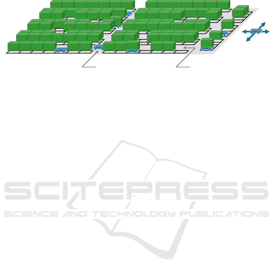
Figure 1: Example of an RMFS.

because vehicles are costly and too many could be

unprofitable (Vis, 2006).

In this paper, we describe a case study involving

an RMFS. We use a simulation model, which we

validate analytically. Simulation experiments reveal

reachable throughput as a function of the number of

vehicles, taking blocking effects among them into

account. We are thus able to show the implications

of blocking effects on the usability of static analytic

approaches for throughput calculation.

We further investigate the influence of different

layout configurations to answer the following

questions:

 Is using two lanes (one for each direction) within

each storage aisle to achieve more throughput

worth the significantly greater space required?

 Is assigning a direction to each single-lane

storage aisle helpful or should bidirectional

traffic be allowed instead?

 What is the influence of cross-aisles? They

provide more flexible vehicle-routing options.

However, do they hence lead to greater

throughput due to less congestion?

The remainder of the paper is organized as follows:

We first briefly review the literature on research to

date into determining the optimal fleet size for

AGVSs. We subsequently describe the considered

RMFS in more detail before we present the

simulation model used for the study. In section five,

we describe the simulation experiments conducted

and discuss their results in section six.

2 LITERATURE REVIEW

To determine the optimal AGV fleet size, several

factors have to be taken into account besides the

number of transports. These include, for instance,

the vehicles’ speeds, loading and unloading times,

the system’s layout, traffic congestion, and vehicle-

dispatching strategies. (Müller, 1983).

Both Ganesharajah et al., and Vis provide

literature reviews concerning approaches to fleet-

size determination, which comprise deterministic

and stochastic methods. (Ganesharajah et al., 1998;

Vis, 2006).

A lower bound for the fleet size of an AGVS can

be obtained by dividing the total travel time by the

length of the planning horizon. The total travel time

includes time for loading and unloading, loaded

travel and empty travel. Empty travel occurs when

the next transport task’s starting point differs from

the previous task’s completion point. The loaded

travel time can be calculated using the From-To

chart, assuming that AGVs travel the shortest path to

complete their assignments. In reality, conflicts with

other AGVs may cause an AGV to take a longer

path. (Ganesharajah et al., 1998)

Additionally, getting the From-To chart becomes

increasingly difficult with a rising number of

possible start points and ends of an assignment. If

AGVs operate in an RMFS, assignments can lead

from any storage location or picking station to any

other. The associated From-To chart comprises one

value for each pair of start and end points. Instead of

calculating each individual travel time, one can use

the mean travel time between a picking station and

any storage location, or between two storage

locations, respectively. This approach has been

applied to storage and retrieval systems for many

decades. As it neglects blocking effects between

AGVs, it has to be considered a static approach.

(Großeschallau, 1984; Gudehus, 2010)

The influence of vehicle-dispatching rules makes

estimating empty-travel time a complex task.

Malmborg presents an analytical procedure to

estimate empty-vehicle travel volume considering

different dispatching rules. (Malmborg, 1991)

Additionally, the more vehicles are moving

within the system, the more blocking among them

will occur (Schmidt, 1989). Static approaches are

insufficient to quantify these blocking effects. A

simulation study has to be conducted instead. Scant

cross-aisles

storage aisle

picking area

SIMULTECH 2018 - 8th International Conference on Simulation and Modeling Methodologies, Technologies and Applications

384

literature exists on RMFS fleet size. Lamballais et

al., analyze the performance of RMFS with and

without storage zones serving single-line and multi-

line orders. They use an analytic approach based on

a queueing network model to estimate maximum

order throughput, average cycle time, and vehicle

utilization. For modelling, they assume that aisles

allow only unidirectional travel and that no vehicle

blocking or congestion occurs in the aisles.

(Lamballais et al., 2017)

Yuan and Gong use a queueing network model

as well to compare different strategies for RMFSs.

They compare the performances of pooled and

picker-dedicated vehicles and calculate the optimal

number and velocity of the vehicles. (Yuan and

Gong, 2017)

The literature mentioned above shows that there

exist different analytical approaches for estimating

the number of vehicles. But as Le-Anh and de

Koster mention, impractical assumptions in the

analytical models may cause the estimated number

of vehicles to differ considerably from that really

needed. A simulation modelling specific operational

conditions should therefore be used to reevaluate the

estimated number. (Le-Anh and De Koster, 2006).

The complex nature of the issues involved in

determining fleet size seems to make simulation the

most promising tool. (Ganesharajah et al., 1998).

Finally, we would like to emphasize why we are

analyzing different layout configurations regarding

direction of travel within the storage aisles.

According to Le-Anh and De Koster, the way in

which vehicles travel through the system

(unidirectional or bidirectional) influences vehicle-

fleet size. (Le-Anh and de Koster). The main reason

for unidirectional traffic is simplicity of layout

design and traffic control. But as Egbelu and

Tanchoco showed by simulation, the use of

bidirectional traffic can increase productivity,

especially if fewer vehicles are required (Egbelu and

Tanchoco, 1986).

3 CONSIDERED SYSTEM

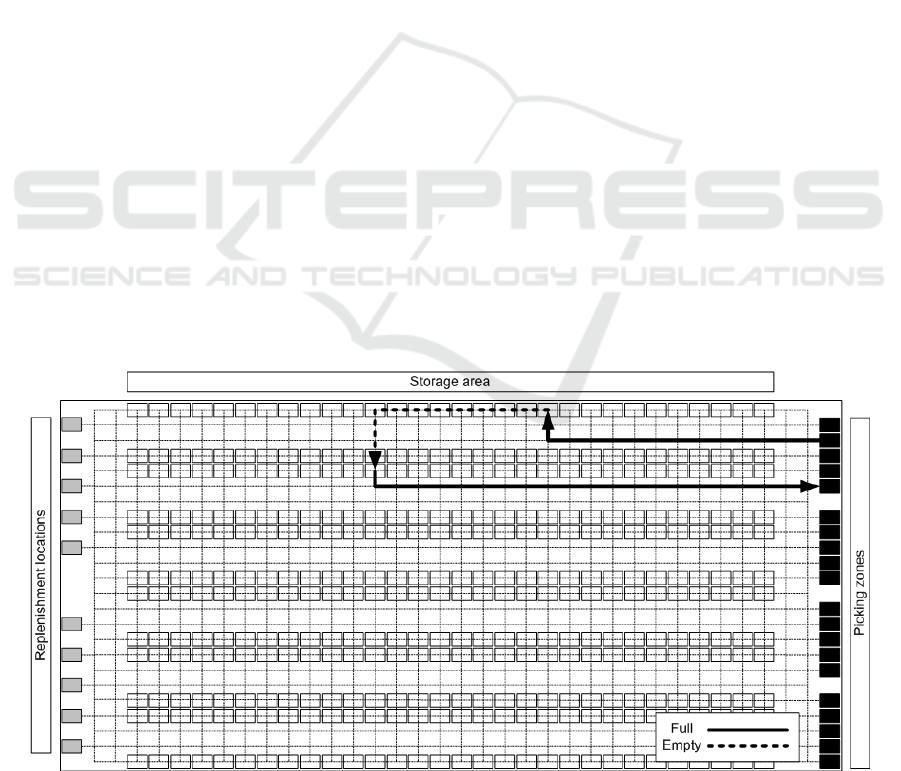
Figure 2 shows the investigated RMFS’s basic

layout (floor plan). The white boxes represent the

stored items placed on small racks, further called

storage units. These storage units are assembled into

twelve horizontal rows with six aisles for vehicle

movement in between. Each row is thirty storage

units long. The picking zones are located on the

layout’s far right side. Each of the four zones has

five picking locations (black boxes) where the

storage units are placed during the picking process.

On the layout’s far left side, there are ten

replenishment locations (gray boxes). If a storage

unit becomes empty during picking, it is brought to

one of these locations for replenishment before

being stored again. Dotted lines in the layout

indicate possible AGV movement paths. Two lanes

are apparent within the aisles, between the

replenishment locations and the storage area, and

between the picking zones and the storage area. All

lanes are unidirectional in opposite directions.

The different vehicles are all equally and

permanently assigned to one of the picking zones

Figure 2: Floor plan of the investigated RMFS with a sample dual cycle.

Simulation-based Performance Analysis in Robotic Mobile Fulﬁlment Systems - Analyzing the Throughput of Different Layout

Conﬁgurations

385

(picker-dedicated). Thus, they start their cycle at

one of their assigned picking zone’s picking

locations and end it at one picking location in the

same zone. The same applies to the storage units,

which are always stored into the aisle from which

they were earlier retrieved. The items are randomly

distributed (chaotic storage).

The AGVs perform three different cycles to

maintain material flow between storage locations,

picking zones, and replenishment locations. The first

and most common is the dual cycle. The AGV loads

its current picking location’s storage unit, transports

it to a random empty storage location in the same

aisle from which it was earlier retrieved, and stores

it there. Now a new storage unit is randomly

selected. The AGV moves to the selected location,

loads the unit, and transports it to an empty picking

location. The dual cycle with empty rack

commences if the storage unit is empty after the

picking process. In this cycle the empty storage unit

is transported to an empty replenishment location

(preferably one in the same layout half—top or

bottom—as the current picking zone). Afterwards a

new storage unit is gathered and transported to the

picking location. The last cycle consists of three

phases and is therefore called the triple cycle. It is

executed if a storage unit has been replenished and is

waiting to be stored again into the same aisle from

which the new storage unit must be retrieved. In this

case, the storage unit of the current picking location

is stored into a random empty location in its

assigned aisle, the storage unit of the replenishment

location is retrieved and stored into its assigned

aisle, and the new storage unit of the same aisle is

gathered and transported to the picking location.

The described cycles generally apply to all

numbers of vehicles. However, there are small

differences in the AGVs’ controls if there are four or

fewer as opposed to five or more per picking zone.

In the case of four or fewer AGVs, the vehicles

move underneath the storage unit that will be picked

next after they’ve brought a storage unit to the

picking location. With five or more AGVs, the

vehicles do not change their storage units at the

picking station. Instead, they wait until the picking

process for the current storage unit is finished and

store that unit afterwards. If more than five AGVs

are assigned to one picking zone, they have to check

whether there is an empty picking location at their

assigned picking zone after loading the new storage

unit at its storage location. Only then do they move

to this location. If not, they wait at the current

storage location until a picking location becomes

empty. We thus avoid vehicles blocking the main

aisle while they wait in front of the picking stations.

The picking process itself works according to the

principle of “first come, first served.” Therefore, the

storage unit that arrives first at the picking zone gets

picked first.

For the different tasks within the RMFS (picking,

replenishment, loading/unloading of storage items),

various times spans are needed. They are listed in

Table 1.

The picking time is set to a relatively short time

span to prevent the picking process from limiting the

system, since the intent in this paper is to investigate

maximum throughput based on the AGVs. Table 1

also gives the mean speed of the AGVs horizontally

and vertically. Acceleration and deceleration are not

taken into account. The vehicle’s wheels must be

rotated to change the direction of motion from

vertical to horizontal or from horizontal to vertical.

The corresponding time span is also listed in Table

Table 1: RMFS parameters.

Picking

ime 5 s

Replenishment

ime 100 s

Unloading

ime 5 s

AGV speed horizontally

vertically 0.5 m/s

AGV turning

ime 5 s

Although the considered system features some

specific aspects such as control at the picking zone,

it is mostly standard. Only one in 20 picks empties a

bin, which causes 5 % of all cycles to be dual cycles

with an empty rack and another 5 % of all cycles to

be triple cycles. Most of the cycles in a layout with

parallel aisles are thus standard dual cycles.

Moreover, whether a vehicle changes picking

location only accounts for short times in comparison

to the whole cycle time.

4 SIMULATION MODEL

To answer the questions in the scope of this paper,

we follow the typical approach of simulation studies,

which is to derive a conceptual model from the

system under consideration and to translate it into a

computerized model. (Rabe, 2008)

The simulation model consists of four modules

for different functions that establish a transparent,

adaptive and reusable structure: the assignment,

routing, evaluation, and layout modules. Whenever

an AGV needs a new assignment, a request is passed

to the assignment module. The answer comprises the

order of pick stations, storage locations, and a

possible supply location that the AGV has to visit

during the cycle.

SIMULTECH 2018 - 8th International Conference on Simulation and Modeling Methodologies, Technologies and Applications

386

The routing module takes over when the AGV

starts the cycle’s next phase. It calculates the fastest

route between start and end points of this section,

e.g., between pick station and the storage location

where the picked item has to be stored. To find the

fastest route, we apply the Time Window Routing

Method (Lienert and Fottner 2017). Not only is this

method guaranteed to find the fastest route relative

to the currently planned routes of other AGVs, but it

does so without the risk of causing deadlocks. The

whole AGV system can collapse due to an infinite

blockage if deadlocks are not reliably excluded. In

case of single-lane bidirectional storage aisles, for

example, a deadlock occurs if two loaded AGVs

meet each other driving in opposite directions. As

they cannot simply “switch” places, the aisle as well

as both AGVs are blocked if the control can’t

resolve the situation.

To apply the Time Window Routing Method, the

layout has to be modelled as a graph. The graph’s

nodes represent picking, replenishment, and storage

locations as well as aisles and cross-aisle

intersections.

Both the assignment module and the routing

module are connected to the layout module. It

consists of AGVs, storage locations, aisles, picking

stations, and supply locations according to the

system described above. The resulting computerized

model is implemented in Tecnomatix Plant

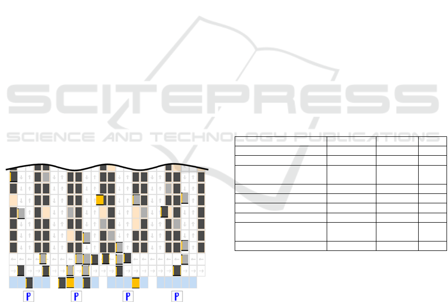
Simulation 11. Figure 3 gives an impression of the

area around the picking locations and part of the

aisles in the computerized model.

Figure 3: Screenshot from the simulation model. Every

rectangle represents a node in the underlying layout graph.

The evaluation module monitors the RMFS’s

behavior with relevance for the performance figures.

Thus, it collects, processes, and stores data from

consecutive experiments and allows for a thorough

evaluation with regard to the questions in the scope

of this paper.

Before conducting experiments, the simulation

model has to be verified and validated. We first use

a structured walkthrough to prove that our model’s

implementation is free of mistakes and thus can be

regarded as verified. In a second step, we compare

the cycle times of AGVs in our simulation model

with those from the static analytical approach to

calculate mean cycle times (see Großeschallau, 1984

or Gudehus, 2010). As this analytical approach does

not take into account blocking effects, we use a

single AGV to conduct dual cycles, dual cycles with

an empty item, and triple cycles randomly using all

possible picking stations, storage locations, and

supply locations. We also consider the empty travel

time between two picking stations in case of five or

more AGVs and single-lane bidirectional aisles (see

Section 3). To calculate cycle times analytically, we

split the cycle into time needed for turning,

loading/unloading and into segments of one-

dimensional, constant travel. Although turning and

loading/unloading are easily counted, the segments’

travel times depend on mean length and the AGV’s

velocity. The cycle time is then composed of these

components. The comparison of calculated and

simulated cycle times shows that the deviation

reaches a maximum of 1 %, which is acceptably low

(cf. Table 2). The simulation model is thus regarded

as valid.

Table 2: Validation of cycle times.

Calculation Simulation Delta

–

4 AGVs

Dual cycle 244 s 245 s 0 %

Dual cycle with empty

items

309 s 306 s 1 %

Triple cycle 392 s 394 s 0 %

5+ AGVs

Dual cycle 225 s 225 s 0 %

Dual cycle with empty

items

289 s 286 s 1 %

Triple cycle 372 s 374 s 0 %

5 EXPERIMENTS

The validation results show that a comparison

between simulation and static analytical calculation

is only possible for basic cycles of a single AGV.

Blocking effects as well as different layout

configurations are beyond the scope of analytical

models. But using our verified and validated

simulation model, we can include both aspects and

run experiments to find out more about how each

affects the system. In the experiments, we compare

Simulation-based Performance Analysis in Robotic Mobile Fulﬁlment Systems - Analyzing the Throughput of Different Layout

Conﬁgurations

387

three different layouts. Layout 1 corresponds to the

current system layout with two unidirectional lanes

per aisles. Layout 2 only provides a single lane per

aisle that can be used in both directions, whereas

Layout 3 allows only unidirectional traffic along a

single lane per aisle (cf. Figure 4). Furthermore, we

investigate the performance of each layout with and

without cross-aisles. We use two cross-aisles located

at one third and at two thirds of the aisle length.

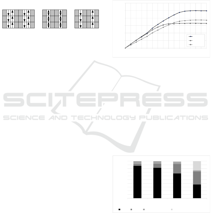
Figure 4: Section with two lanes for a) Layout 1, b)

Layout 2 and c) Layout 3.

With each layout, we vary the number of

vehicles from four (one per picking zone) to 60 (15

per picking zone) in steps of four. Simulation time is

set to 24 hours and a simulation run is repeated ten

times with each setting.

6 RESULTS

In this section, we present and discuss the results

obtained by the simulation. Figure 5 provides an

overview of the results without cross-aisles. The

curves look similar for all three layouts, and we will

see that this holds for cross-aisles as well (cf. Figure

3). In all cases, performance scales nearly linearly

with the number of vehicles until it reaches

saturation. The curves show a small knee between

16 and 20 vehicles or four and five vehicles per

picking zone, respectively. This is where the cycles

change as AGVs do not have to change the picking

location anymore between arrival and departure. As

soon as the saturation begins, the gain per additional

vehicle decreases to zero. At this stage, more

vehicles within the system do not further increase

performance. Blocking effects caused by the

additional vehicles result in a loss of performance

across all vehicles, which exactly counterbalances

the additional vehicles’ performance contributions.

A look at the time spans that the AGVs spent on

different activities helps to prove this.

Figure 6 shows

these amounts for Layout 2. There are four possible

activities: driving, loading and unloading, waiting

blocked during driving, and waiting loaded at a

storage location until a picking location is ready for

the next item. The last activity only occurs when

there are six or more vehicles per picking zone, as

each picking zone only provides picking locations

for five vehicles simultaneously. The increasing

amount of waiting due to blocking reflects the

blocking effects. With 60 vehicles in the RMFS, a

third of the time is spent blocked, whereas minor

blocking occurs with eight and 16 vehicles and

throughput rises linearly with the number of

vehicles.

Figure 5: Throughput of all three layouts without cross-

aisles.

Layout 1 provides the greatest throughput, which

one would expect due to two unidirectional lanes per

aisle. It is remarkable, however, that for fewer

vehicles, Layout 2 outperforms Layout 3. The

former’s aisles can be used in both directions, which

shortens the calculated paths. The more vehicles are

working within the system, the heavier the

congestion becomes. After a certain number of

vehicles is reached, allowing only unidirectional

traffic—as in Layout 3—is beneficial. Doing so

requires no changes in the physical layout and offers

a promising way to increase throughput using

control measures alone if insufficient space is

available to use Layout 1.

Figure 6: Amounts of time spent per AGV during the four

possible activities.

The second layout feature we tested is the

existence of cross-aisles that enable vehicles to

switch aisles not only in the front and back of, but

)c)

100

200

300

400

500

600

0 4 8 12162024283236404448525660

Cycles per hour

Number of AGVs

Layout 1

Layout 2

Layout 3

10%

20%

30%

40%

50%

60%

70%

80%

90%

100%

8 163260

Amount of time

Number of AGVs

driving blocked loading & unloading waiting at storage location

SIMULTECH 2018 - 8th International Conference on Simulation and Modeling Methodologies, Technologies and Applications

388

also at regular distances along the aisles.

Figure 3

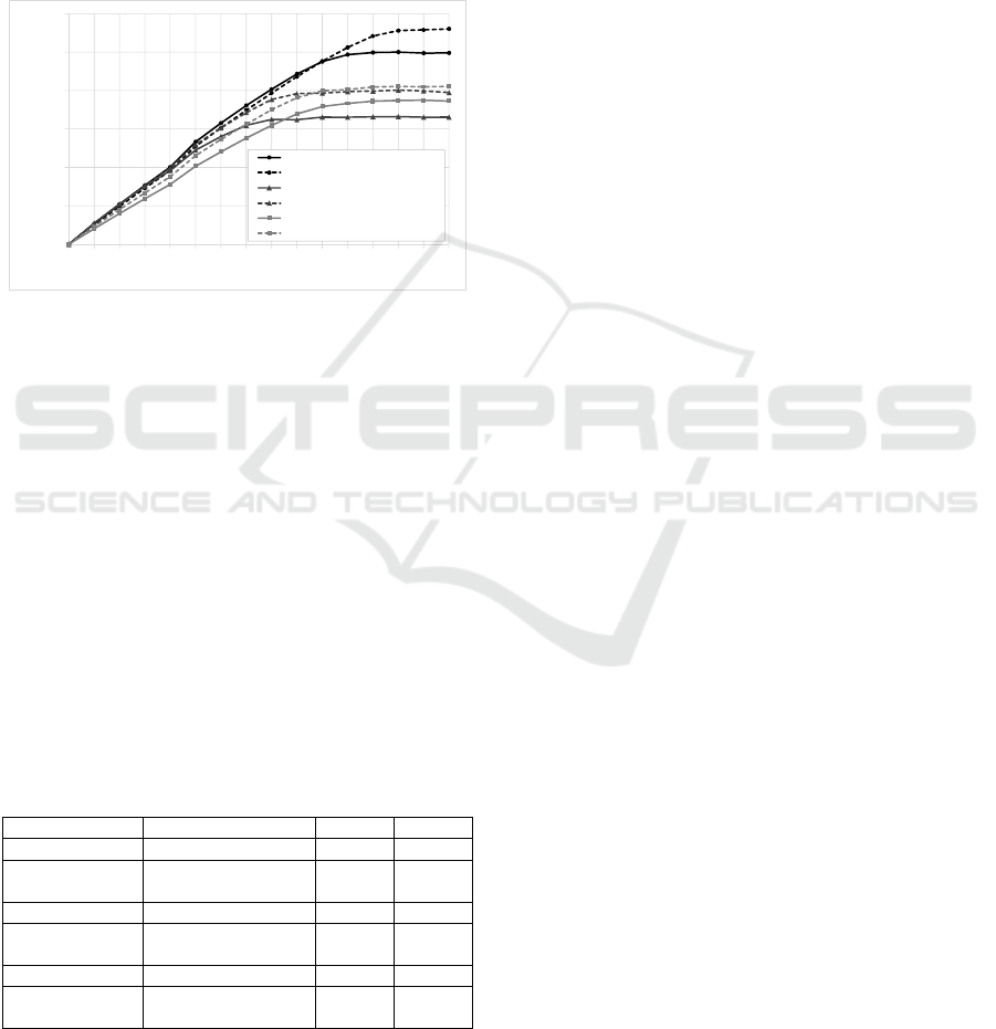
compares the throughputs of the different layouts

with and without cross-aisles. As mentioned above,

all curves look similar with a linear increase and a

small knee between 16 and 20 vehicles before

reaching saturation. Cross-aisles help to increase

throughput for every layout. The larger number of

routing options reduces blocking effects as expected.

Vehicles can more easily circumvent congested parts

of the layout thereby smoothing traffic.

Figure 7: Throughput of all three layouts with and without

cross-aisles.

Table 3 provides an overview of the maximum

throughput per layout and the number of AGVs that

was needed to reach that throughput. We define

maximum throughput as the first throughput that

increases less than one percent with the addition of

one vehicle per picking zone. Furthermore, the

differences in number of nodes within the storage

area is given with Layout 1 as reference. For

instance, Layout 1 with cross-aisles provides a

significantly greater throughput, but requires 26.7 %

more aisle nodes than Layout 1 without cross-aisles

does, whereas Layout 3 with cross-aisles achieves

less throughput (90 fewer cycles per hour) but

requires 40 % fewer aisles nodes.

Table 3: Comparison of performance and space

requirements.

Max. cycles per hour AGVs Nodes

Layout 1 489.9 48 -

Layout 1 with

cross-aisles

556.2 52 +26.7 %

Layout 2 324.7 32 −50.0 %

Layout 2 with

cross-aisles

391.8 36 −40.0 %

Layout 3 372.3 48 −50.0 %

Layout 3 with

cross-aisles

409.0 48 −40.0 %

From the curves in Figure 7, one can figure out

how many AGVs are needed to reach a certain

throughput. Furthermore, they hint at whether a

static approach that does not take blocking into

account also holds. For example, if a throughput of

200 cycles per hour is needed, the curves of all six

layouts are in the linear section. A static approach is

thus applicable. For a throughput of 450 cycles per

hour, however, a static approach results in a fleet

size of about 36 to 48 vehicles for the different

configurations. These numbers can be roughly

estimated by extrapolating the linear parts of the

curves up to 400 cycles per hour. The simulation,

however, shows that Layouts 2 and 3 reach

saturation below 450 cycles per hour. The system

would be unable to reach the desired throughput if

these layouts were chosen.

7 CONCLUSIONS

In this paper, we considered a robotic mobile

fulfilment system with six storage aisles, four

picking zones, and ten replenishment locations. We

conducted a series of simulation experiments to

compare the performances of different layout

configurations. We varied the number of vehicles

and analyzed the throughputs reached.

A bidirectional single lane layout is

recommended for fewer vehicles. However,

maximum throughput is reached with two

unidirectional lanes per aisles, although this layout

requires the most space. Using cross-aisles generally

yields greater throughput.

We were able to show that the more vehicles are

working within the system, the less throughput each

additional vehicle provides. For fewer vehicles, the

throughput is nearly a linear function of the number

of vehicles. Here it is admissible to analyze the

throughput of a single vehicle analytically and

forecast the throughput for more vehicles. But the

analytical approach underestimates the required

number of vehicles as soon as increasing blocking

effects among vehicles causes departure from

linearity. The crucial point is that numbers of

vehicles for which linearity holds is unknown. The

completion of a simulation study is therefore

essential for obtaining reliable performance results.

Based on this conclusion, we identify two

possible fields of future research: First, the scope of

the simulation model has to be extended towards

other aspects of planning like different storage

policies and dispatching rules. Both influence the

vehicles‘ travel distances and system performance.

Additionally, we assumed that the vehicles are

available without restrictions. However, battery

100

200

300

400

500

600

0 4 8 12 16 20 24 28 32 36 40 44 48 52 56 60

Cycles per hour

Number of AGVs

Layout 1

Layout 1 - with cross-aisles

Layout 2

Layout 2 - with cross-aisles

Layout 3

Layout 3 - with cross-aisles

Simulation-based Performance Analysis in Robotic Mobile Fulﬁlment Systems - Analyzing the Throughput of Different Layout

Conﬁgurations

389

management and emergency policies in case of a

vehicle break down affect the system performance.

Using our simulation model, the effects of both can

be analyzed during planning.

Second, to generalize our findings, a next step

can be to analyze at which number of vehicles the

performance starts to deviate from the linear,

analytical curve. If that is the case at a similar ratio

of vehicles per area in different layouts or layout

sizes, it would be an indication on whether a

simulation study has to be conducted. For systems

with an analytically calculated number of vehicles

around this ratio or higher, planners would have a

rule of thumb of when to reevaluate their findings

with a simulation.

REFERENCES

Boysen, N., Briskorn, D., Emde, S., 2017. Parts-to-picker

based order processing in a rack-moving mobile robots

environment. European Journal of Operational

Research 262 (2), pp. 550–62.

Egbelu, P.J. and Tanchoco, J.M.A.,1986. Potentials for bi-

directional guide-path for automated guided vehicle

based systems. International Journal of Production

Research 24 (5), pp. 1075–10097.

Ganesharajah, T., Hall, N.G., Sriskandarajah, C., 1998.

Design and operational issues in AGV-served

manufacturing systems. Annals of Operations

Research 76 (0), pp. 109–54.

Großeschallau, W., 1984. Materialflussrechnung –

Modelle und Verfahren zur Analyse und Berechnung

von Materialflusssystemen, Springer. Berlin.

Gudehus, T., 2010. Logistik – Grundlagen Strategien

Anwendungen, Springer. Berlin, 4

edition.

Lamballais, T., Roy, D., De Koster M.B.M., 2017.

Estimating performance in a Robotic Mobile

Fulfillment System. European Journal of Operational

Research 256 (3), pp. 976-990.

Le-Anh, T., De Koster M.B.M., 2006. A review of design

and control of automated guided vehicle systems.

European Journal of Operational Research 171 (1),

pp. 1–23.

Lienert, T., Fottner, J., 2017. Development of a generic

simulation method for the time window routing of

automated guided vehicles. In: Tagungsband 13.

Fachkolloquium der WGTL. WGTL.

Malmborg, C.J., 1991. Tightened analytical bounds on the

impact of dispatching rules in automated guided

vehicle systems Applied Mathematical Modelling 15,

pp. 305–11.

Müller, T., 1983, Automated Guided Vehicles, Springer.

Berlin, Heidelberg, New York, Tokyo.

Rabe, M., Wenzel, S., Spieckermann, S., 2008.

Verifikation und Validierung für die Simulation in

Produktion und Logistik, Springer. Berlin.

Schmidt, F., 1989. Komplexe Fahrerlose Transportsys-

teme – Fahrzeuganzahl, Investitionsaufwand, Wirt-

schaftlichkeit, Verlag TÜV Rheinland. Köln.

VDI-Richtlinie 2510, 2005. Automated Guided Vehicle

Systems. Beuth. Berlin.

Vis, I.F.A., 2006, Survey of research in the design and

control of automated guided vehicle systems.

European Journal of Operational Research 170 (3),

pp. 677-709.

Yuan, Z., Gong, Y.Y., 2017. Bot-In-Time Delivery for

Robotic Mobile Fulfillment Systems. IEEE

Transactions on Engineering Management 64 (1), pp.

83-93.

SIMULTECH 2018 - 8th International Conference on Simulation and Modeling Methodologies, Technologies and Applications

390