Analysis of the GNSS Error Distribution

for the Generation of a Cooperative Environment Model

for Advanced Driver Assistance Systems

Florian Alexander Schiegg

1,2

, Tobias Frye

1,2

and Florian Wildschütte

Institute of Communications Technology, Leibniz University of Hannover, Appelstraße 9A, Hannover, Germany

Robert Bosch GmbH, Corporate Research, Robert-Bosch-Strasse 200, Hildesheim, Germany

Keywords: GNSS-Positioning, Localization Accuracy, V2x-Communication, Congestion Control.

Abstract: In the context of rising traffic automation, the generation of a reliable environmental model plays a key role.

By sharing their information, vehicles and infrastructure are able to set up cooperative environmental models

of considerably increased accuracy. The GNSS-based localization receives special attention in this regard,

since it allows switching from vehicle relative coordinates to absolute and vice versa. While the focus of most

related work lies on improving the mean of the GNSS fix, the work at hand analyses its error distribution.

Field tests were performed on various scenarios and compared with simulations. Finally, a utility function is

proposed, revealing the amount of information carried by every description parameter of the respective

distribution.

1 INTRODUCTION

The ongoing trend towards automation on the streets

has come along with the need for increasingly

accurate environmental models. In this context

vehicle to infrastructure (V2I) and vehicle to vehicle

(V2V) communication have received growing

interest in the past years. They allow to improve the

environmental model obtained from the vehicles’

own on-board sensors by fusing it with data from the

incoming V2X-messages.

Sensor measurements, however, are faulty and

every object’s state is associated with a certain error

distribution. Fusion algorithms, like the Kalman

filter, heavily rely on an accurate estimation of these

errors to weight the data of the different sensors. Also,

the association of a measurement to a specific object

within the environmental model is done based on the

estimation of its associated error.

The GNSS localization receives special attention

in the V2X context, since the information shared has

to be transformed from the emitting vehicle’s relative

coordinates to absolute and later back to the receiving

vehicle’s coordinates. Hence, due to error

propagation, all transmitted data is subject not only to

the underlying sensors’ intrinsic precision, but also to

the absolute localization errors of both vehicles. An

exact estimation of the GNSS positioning error is thus

of utmost importance.

In this work, different error estimations of the

GNSS-based localization are compared. Based on

these results, a utility function for the information

content of every additional description parameter is

set up, and the plausibility of the results is finally

investigated by means of Monte Carlo simulations.

2 STATE OF THE ART

While there are a vast variety of proposed localization

methods, the literature aimed at the estimation of its

accuracy is considerably scarcer. Pullen, Walter, and

Enge (2011) address the need for adapting existing

integrity concepts from specific risk (e.g. aviation) to

average risk applications (e.g. train and automotive).

Since most receivers only write out specific sentences

of the NMEA 183 standard defined by the National

Marine Electronics Association (2008), a generic

approach is needed to estimate the localizations error

distribution (e.g., Cosmen-Schortmann et al., 2008;

Mahdia et al., 2015). For its applicability in the

automotive sector, the estimation has to be feasible in

real time (e.g., Streiter et al., 2012 & 2013; Margaria

& Faletti, 2014; Mahdia et al., 2015). It would further

Schiegg, F., Frye, T. and Wildschütte, F.

Analysis of the GNSS Error Distribution for the Generation of a Cooperative Environment Model for Advanced Driver Assistance Systems.

DOI: 10.5220/0006793805450551

In Proceedings of the 4th International Conference on Vehicle Technology and Intelligent Transport Systems (VEHITS 2018), pages 545-551

ISBN: 978-989-758-293-6

545

be desirable to take into account shape-information

about the error distribution comprised by the satellite

constellation (e.g., Kaplan, 2005; Margaria and

Faletti, 2014). This work attempts to cope with these

issues simultaneously.

3 METHODOLOGY

This section describes the methods employed

throughout this work. Section 3.1 briefly introduces

the employed mathematical models and the

evaluation of the results. The data collection is then

described in section 3.2.

3.1 Theoretical Background

3.1.1 Horizontal Dilution of Precision

As mentioned previously, the constellation of the

satellites used for the localization contains

information concerning the shape of the positioning-

error. The error vector can be written as (Kaplan,

2005):

=H





(1)

where  represents the pseudorange error and













,,,

2,2,2,

1,1,1,

kzkykx

zyx

uuu



(2)

is a matrix composed of the satellite positions relative

to the GNSS receiver





,



,



,

=

sin

(







)

cos(



)

cos

(







)

cos(



)

sin(



)



(3)





and 



are the azymuth and elevation of the k-

th satellite respectively. The covariance can then be

obtained from the expected value of the error vector:



(



)









(4)

By introducing Eq. 1 into Eq. 4 one then obtains



(



)

(









)





()=

(



)









(5)

In the second step 

(



)

=





was assumed to

be constant. This approach assumes a multivariate

Gaussian distribution of the error vectors and is often

utilized in literature for its good results and

simplicity. 





is the so-called user equivalent

range error that describes the error contributions from

the ionosphere, troposphere, multipath propagation,

receiver noise, clock and ephemeris, and usually takes

values between 0.5m and 10m depending on the

quality indicator of the used receiver. A deeper

treatment is offered by Kaplan (2005). While the user

equivalent range error is a mere factor, the matrix

(



)















44434241

34333231

24232221

14131211

DDDD

(6)

contains the information about the errors shape. It is

called the dilution of precision (DOP) matrix.

3.1.2 Error Morphologies

The upper left 2x2 part of the DOP matrix contains

all relevant information about the 2D localization

error. For symmetry reasons, it consists of only three

independent parameters. By simple math it is possible

to obtain the characteristic ellipse-shaped confidence

intervals of the bivariate-Gauss-distribution (red area

in Fig 1).

Figure 1: Error estimation morphologies.

In some cases, the system can be satisfactorily

described by two parameters. For instance, for some

applications only the error parallel and perpendicular

to the driving direction C is of interest. This is usually

the case when the GNSS data stays on-board and is

not transmitted to the surrounding V2X-capable

traffic objects. The DOP matrix is then transformed

to the ego-coordinate system of the GNSS receiver

and the resulting correlation terms are set to zero,

VEHITS 2018 - 4th International Conference on Vehicle Technology and Intelligent Transport Systems

546

resulting in an ellipse aligned with the driving

direction (green area in Fig. 1).

For terrestrial applications, often only one

parameter, the so-called horizontal dilution of

precision (HDOP) is considered (Betz, 2016). It can

be computed as

=







+



(7)

Multiplied by the UERE, it gives an estimation of the

radius of a circle-shaped error distribution (blue area

in Fig. 1).

For simplicity’s sake the introduced error

distributions will further be referred to by the number

of their description parameters (e.g. the circle would

be called the 1 parameter ellipse (1PE)).

3.1.3 Evaluation

To obtain a sufficiently accurate environmental

model it is crucial to know which error estimate is

most suitable for each scenario. Further, it would be

desirable to determine how much information is

carried by each supplementary description parameter

to provide some sort of utility function and herewith

allow a case specific evaluation of the parameters to

be transmitted.

In order to make the error distributions

comparable it has to be made sure they all represent

the same confidence interval. For three main reasons

the empirical UEREs supplied by literature are

insufficient in this regard: (i) The UEREs vary

significantly between different sources, (ii) the

elimination of the correlation terms and the resulting

diverging areas of the different error estimations

imply modified confidence intervals, and (iii) the

localization error is sensitively dependent on the

algorithms and hardware employed by each GNSS

receiver.

Hence, the UERE must be adjusted for each

distribution in a way that it correctly predicts an equal

number of measurements. This done, the estimations

can finally be compared based on the proportion of

estimations they do best and the average area

necessary to meet the described normalization

requirements. The latter is particularly important

since it yields the accuracy of a model in form of its

resolution.

3.1.4 Monte Carlo Simulations

Assuming the error distribution is completely random

and thus uncorrelated to the inclination angle of the

3PE, then statistically 50% of the measurements

would lie up to 45° away from its major axis. In other

words, in half of the cases the ellipse would describe

the error more precisely than the circle. On the other

side, should the error distribution be perfectly

described by the covariance matrix, then the amount

of situations the 3PE predicts the error in a better way

depends on its deformation. Fig. 2 shows an ellipse

with deformations a) =1.3 and b) =2.0

representing a random confidence interval of the error

distribution. It is superposed by a circle of the same

area and thus, resolution. Measurements located on

the illustrated straight lines through the intersections

of circle and ellipse will thus be equally well

predicted by both geometries with equal resolution.

On these lines, the Mahalanobis-distances of both

models would also be alike. It can be noted that the

Mahalanobis-distance of a 3PE is smaller in the red

area than that of the 1PE and vice-versa for the blue

area.

Figure 2: Region where the 1PE (blue) and the 3PE (red)

require lower UEREs to describe the error for an ellipse

deformation of a) =1.3 and b) =2.0 respectively.

Similar thoughts apply for the expected relative

resolution of the estimations and the 2PE. Making use

of Monte Carlo simulations it is hence possible to

numerically predict how well the investigated models

should describe the actual data, assuming either a

fully random distribution or one perfectly described

by the DOP matrix. Comparing these theoretical

values with the experimental results makes it possible

to draw conclusions on the nature of the real error

distribution.

3.2 Experimental Setup

Experiments were carried out to investigate the

performance of the proposed error estimates. To this

purpose a test vehicle equipped with an ADMA-g Pro

as ground truth reference was used to collect data on

over 100 km in different scenarios (urban,

countryside and highway). The measurements were

)=.

)=.

Analysis of the GNSS Error Distribution for the Generation of a Cooperative Environment Model for Advanced Driver Assistance Systems

547

performed with two different test receivers, namely

an Adafruit Ultimate GPS (MTK3339 chipset) and a

u-blox EVK-M8T (NEO/LEA-M8T chipset). For

further diversification SBAS was activated only on

the former. All in all, over 45000 localizations were

carried out (Table 1).

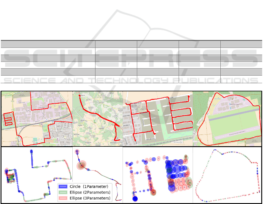
Table 1: Description of the investigated tracks.

Track Scenario Receiver Distance

Mixed Adafruit 10.9 km

Mixed Adafruit 5.2 km

Highway Adafruit 27.2 km

Mixed Adafruit 6.1 km

Highway Adafruit 39.1 km

Country Side u-blox 12.1 km

Mixed u-blox 9.2 km

Urban u-blox 3.3 km

4 RESULTS AND DISCUSSION

4.1 Data Characterization

A characterization of the measurements for both test

receivers and in distinct scenarios is provided in table

2. Interestingly the average horizontal error of the u-

blox presented significantly lower values than the

Adafruit with activated SBAS. Even in strongly

screened areas it was able to detect a larger amounts

of satellites, resulting in only moderately deformed

ellipses (~1.26).

It is worth noticing that the Adafruit lost

connection on a segment of the highway, yielding

either no fix or extremely high errors (Fig. 4b). Since

the overall average is of interest and this situation is

not uncommon, these points were not filtered out.

Further, the used test receivers employ internal

correction algorithms that lead to inertial effects on

the vertices of the trajectories, as can be seen in detail

in figure 3. The effect is also well visible in a larger

scale in figure 4a, were the best fitting error

estimation changes briefly after most of the vertices.

Since the vast majority of receivers employ internal

correction algorithms and their influence on the

results cancel out for sufficiently large amounts of

data, the fixes were taken without further

modifications.

4.2 Normalization

In a first step, the exact UERE was determined for

each error estimation (Fig. 3). This means that the

diameter of the geometries was chosen in a way that

the measured fix lies right on its border.

The lower row of figure 4 shows the error estimate

of highest resolution for every measurement. The

only best fitting estimate was amplified by a factor of

10 for better visualization. As can be noted, in all

scenarios the 3PE described the real error more

accurately (lower area) than 1PE and 2PE. It should

be kept in mind that only the portion of fixes best

described by each geometry is of interest in this case,

and not the area. Thus the colours may be a bit

misleading at first sight.

The amount of fixes where the 3PE presented a

lower area than the 3PE ranged from 52% in urban

areas to 78% on the highway. The obtained values are

shown on table 2.

However, since in practice the estimation has to

be made in real time, a fix UERE has to be determined

in advance. Fig. 5a and 5b show the number of

measurements correctly predicted by each

distribution as a function of the chosen UERE for the

Adafruit and the u-blox respectively. As can be seen,

the commonly used 

%

 ranging from 5.0 to

7.1 (Betz et al., 2016; Kaplan, 2005) would contain

only 70-86% of the Adafruit’s but 100% of the

Figure 3: A posteriori calculated exact UEREs for given reference (red) and measurement (blue). The arrows point into the

driving direction.

VEHITS 2018 - 4th International Conference on Vehicle Technology and Intelligent Transport Systems

548

u-blox’s measurements, confirming the necessity of

its readjustment to ensure comparability.

It is worth noticing that even though different

scenarios were analysed with each receiver, the

cumulative error distributions converge in the same

order for both (descending: 3PE, 2PE and 1PE).

4.3 Estimations Accuracies

Once the error estimations are normed to correctly

predict equal numbers of measurements, they can be

compared based on their resolution. As mentioned

before, the resolution of an estimation is proportional

to the inverse of its area. Table 2 summarizes the

mean areas relative to the one of the 3PE at a

confidence interval of 95% for the different scenarios.

As could be expected from the previous results, both

the 1PE and the 2PE require larger confidence

intervals than the 3PE in three of the four investigated

scenarios. Only in urban areas the 1PE seems to be

more accurate. However, by observing Fig. 6b the

large oscillations stand out. It shows the areas of each

distribution relative to that of the 3PE as a function of

the confidence interval estimated with the determined

fix UEREs. The oscillations are attributed to the size

of the analysed sample (as a reference, for the Monte

Carlo simulations to converge over 100 mio.,

simulated localizations were necessary). However,

despite these oscillations the considerably lower

relative performance of the 3PE is clearly visible.

Thus, in areas with higher building density the DOP-

matrix seems to lose validity. This effect may be

explained by multipath propagation on the

surrounding buildings, distorting the DOP matrix and

leading to a more random distribution.

When comparing Fig 6a and 6b, a second effect

can also be appreciated. Better receivers consider

more satellites for their calculations, reducing the

deformation of the ellipses, making them more

similar to circles and reducing the impact of

additional description parameters.

Table 2: Characterization of the collected data. In brackets the theoretical values obtained from Monte Carlo simulations.

Scenario Mixed Highway Urban Rural

GNSS Receiver

Adafruit Adafruit u-blox u-blox

Absolute Error [m]

2.82±1.70 5.19±8.41 1.59±0.65 0.91±0.18

Deformation =/ 1.37±0.11 1.36±0.24 1.26±0.12 1.15±0.09









(exact UERE)

0.67 (0.56) 0.78 (0.55) 0.52 (0.54)

0.66 (0.52)

Rel. Area









[95%]

1.26 (1.06) 1.21 (1.06) 0.96 (1.04) 1.09 (1.02)

Rel. Area









[95%]

1.17 (1.04) 1.04 (1.04) 1.00 (1.03) 1.06 (1.01)

Figure 4: Selection of tracks for the different scenarios (upper row) and best describing error geometry (lower row) for a-

posteriori computed exact UEREs (augmented by a factor of 10 for a better visualization).

)

)

)

)

Analysis of the GNSS Error Distribution for the Generation of a Cooperative Environment Model for Advanced Driver Assistance Systems

549

Figure 5: Cumulative error distributions of a) the Adafruit and b) the u-blox.

Figure 6: Relative mean area of the estimated confidence intervals, a) Adafruit, mixed and b) u-blox, urban.

With the obtained results it is then possible to

partially construct a utility function to estimate the

value of every additional parameter, depending on the

scenario. In strongly shaded regions multipath

randomly scatters the measured fixes of both

receivers, significantly reducing the validity of the

3PE-model. However, in mainly open surroundings

the 2PE was found to be in average 7% (2%) and the

3PE even up to 25% (8%) more accurate than the 1PE

for the Adafruit (u-blox). which is a fairly large

increase. In the ADAS-context an increase of this

magnitude in accuracy presents a considerable

improvement. Three key systems of highly automated

vehicles profit from a more precise estimation of the

localization error: (i) Association: To construct the

environmental model for the ADAS-system to base

its decisions on the objects detected by different

sensors have to be associated. In the case of a

cooperative environmental model, also the objects

transmitted via V2X-communication have to be

associated with those of the local environmental

model. A precise knowledge of the data’s accuracy is

essential. (ii) Sensor fusion: The data of an object

provided by different sensors is then fused, weighted

by the estimated accuracies. A better estimation of the

GNSS localization error thus leads to a better overall

localization after the data is fused with that of other

sensors. (iii) V2X-comunication: On-board sensors

employ a relative coordinate system. To share data

with other V2X-cappable vehicles, this data has thus

to be transformed to absolute coordinates in the

sending vehicle by means of its GNSS-fix and its

accuracy. The receiving vehicle then has to transform

it back to its own coordinate system, making use

again of its absolute position and associated error

estimation. A bad GNSS-error estimation will thus

have a large negative impact on the transmitted sensor

data.

This in mind, the performance increase provided

by the 3PE with respect to the 1PE is thus

considerable. However, it should be noted that the

obtained values have to be taken with the appropriate

caution. As the results showed, the utility function is

VEHITS 2018 - 4th International Conference on Vehicle Technology and Intelligent Transport Systems

550

receiver specific and depends significantly on its

quality.

4.4 Comparison with Simulations

Comparing these observations with the theoretical

values determined by Monte Carlo simulations (listed

in brackets in table 2) shows that in urban areas the

real error distribution lies somewhere between that of

a fully random distribution (ratio 50%) and that of the

covariance matrix (ratio 54%).

Figure 7: Dependence of the predictions performances on

the distributions deformation (Monte Carlo simulations).

All other scenarios lie well above the theoretical

value, proving that the covariance matrix is not only

strongly correlated to the real error distribution in

open sky areas, but also that higher axis ratios would

describe it better with the same inclination angles,

hinting systematic errors. Since this behaviour

occurred equally for varying experimental conditions

(e.g. speed, driving direction, satellite constellations,

daytime, etc.) it can most probably be traced back to

the receivers themselves. Many receivers rely on the

weighted least squares method, which weights the

used satellites independently. In single-frequency

SPS receivers the pseudorange error measurements,

dominated by ionospheric effects, can be

approximated by the satellites’ elevations (Kaplan,

2005, 332). This results in higher deformations of the

error distriutions. The same conclusions apply to the

relative resolution of the analysed error estimations.

5 CONCLUSION

The main purpose of this work was to compare

different error distributions of the GNSS localization

derived from the satellite constellation. Field tests

were performed in characteristic scenarios, at varying

conditions, daytimes, and test receivers. It could be

shown that while shadowing has a positive effect on

the distributions’ eccentricity and thus on the 3PEs

relative accuracy, multipath propagation leads to the

opposite result. The latter could be attributed to the

distortion of the DOP matrix due to satellites

erroneously taken into account. In open sky areas

however, the 3PE estimation proved to perform

considerably better than the simplified error

distributions. Furthermore, the magnitude of this

effect seemed to be correlated to the used test

receiver. Cheaper receivers incorporate fewer

satellites into their fixes, yielding more deformed

error distributions. The gain of accuracy per

transmitted parameter is thus notably higher than in

expensive super accurate receivers. Simulations

supported the experimental results; nevertheless,

further research is highly encouraged.

REFERENCES

Betz John W., 2016. Engineering satellite based navigation

and timing: Global Navigation Satellite Systems, Signals,

and Receivers. Wiley-IEEE Press.

Cosmen-Schortmann, J., Azaola-Sáenz, M., Martínez-

Olagüe, M., & Toledo-López, M., 2008. Integrity in

Urban and Road Environments and its use in Liability

Critical Applications. IEEE/ION Position, Location and

Navigation Symposium.

Kaplan Elliott D., 2005, Understanding GPS: Principles and

Applications. Artech House Publishers, London, 2

edition.

Margaria Davide and Faletti Emanuela, 2014. A novel local

integrity concept for GNSS receivers in urban vehicular

contexts. IEEE/ION Position, Location and Navigation

Symposium.

National Marine Electronics Association (NMEA), 2008,

NMEA 0183 Standard, viewed 1 December 2017,

http://www.nmea.org/

Pullen Sam, Walter Todd, and Enge Per, 2011. SBAS and

GBAS Integrity for Non-Aviation Users: Moving Away

from Specific Risk. International Technical Meeting of

the Satellite Division of the Institute of Navigation.

Streiter Robin, Bauer Sven, Bauer Stefan, and Wanielik

Gerd, 2013. GNSS Correction Services for ITS

Applications: A performance Analysis of EGNOS and

IGS. IEEE Intelligent Transportation Systems.

Streiter Robin, Bauer Sven, Bauer Stefan, and Wanielik

Gerd, 2012. GNSS Multi Receiver Fusion and Low Cost

DGPS for Cooperative ITS and V2X Applications. 9th

ITS Europe Congress.

Tahsin Mahdia, Sultana Sunjida, Reza Tasmia, and Hossam-

E-Haider Md, 2015. Analysis of DOP and its Preciseness

in GNSS Position Estimation. Electrical Engineering

and Information Communication Technology.

Analysis of the GNSS Error Distribution for the Generation of a Cooperative Environment Model for Advanced Driver Assistance Systems

551