Evaluation of Two Solar Radiation Algorithms on 3D City Models for

Calculating Photovoltaic Potential

Syed Monjur Murshed

, Alexander Simons

, Amy Lindsay

, Solène Picard

and Céline De Pin

European Institute for Energy Research, Emmy-Noether Str. 11, 76131 Karlsruhe, Germany

EDF Inc. Innovation Lab, 4300 El Camino Real, Los Altos, CA 94022, U.S.A.

École Supérieure d'Électricité, Plateau du Moulon, 3 Rue Joliot Curie, 91190 Gif-sur-Yvette, France

ESILV - Paris La Défense, 12 Avenue Léonard de Vinci, 92400 Courbevoie, France

Keywords: Solar Irradiance, Algorithms, 3D City Models, Python.

Abstract: Different algorithms are used to calculate solar irradiance on horizontal and vertical surfaces of the 3D city

models. The goal of this paper is to evaluate the hourly solar irradiance calculated by two widely used

algorithms in order to assess photovoltaic (PV) potential of the 3D city models. Both algorithms are

implemented in an open source software infrastructure consisting of PostgreSQL database connected with

PostGIS, Python, etc. The results show a significant variation of solar irradiances on horizontal, vertical and

tilted surfaces. Finally, the justification of a particular algorithm to assess citywide PV potentials is made.

1 INTRODUCTION

Calculation of solar irradiance on horizontal, vertical

and tilted building surfaces helps to correctly estimate

techno-economic photovoltaic (PV) potential, assess

building heating and cooling energy needs (Murshed

et al., 2017; Bahu et al., 2014), identify the Urban

Heat Island (UHI) effects (Vitucci et al., 2014).

Solar energy is one of the environmentally

sustainable resources for producing electricity using

photovoltaic systems (Šúri and Hofierka, 2004).

Different building surfaces are exposed to the sun,

which can be utilized to generate energy by efficient

installation and design of the PV panels. In this

regard, it is important to know the exact irradiance

received by the horizontal, vertical and tilted surfaces.

Moreover, based on the different tilt angles and

orientation of the panels, the same surface may

receive more or less radiation. Several other factors

such as shading, sky condition also influence the

amount of solar irradiance received by a surface.

Numerous algorithms (methods) and tools have

been developed across different climatic conditions to

analyze solar irradiance (Šúri and Hofierka, 2004). A

comprehensive and comparative overview has been

given by Freitas et al. (2015), Catita et al. (2014),

Redweik et al. (2013), Gueymard (2012) The GIS-

based analysis of solar irradiance was also performed

in different spatial-temporal scales and resolution:

from building surfaces to districts, hourly or monthly

basis, using vector or raster data (Huld, 2017; Li and

Liu, 2017; Hachem et al., 2013; Nguyen and Pearce,

2010; Lee and Zlatanova, 2009). However, the use of

3D city models is rather recent and innovative

(Freitas et al., 2015; Wieland et al., 2015). With the

availability of comprehensive 3D building data across

many cities, it is possible to carry out sophisticated

analysis of solar irradiance at a greater detail. It

allows assessing the shadow effect from the

neighbouring buildings, terrain or other urban

objects, calculating slope and orientation of the

surface, etc. Several commercial tools such as

Archiwizard, Rhinosolar, Autodesk Ecotect, ArcGIS

are also available but they are not able to perform

analyses on vertical surfaces or are not suitable to be

used in large 3D city models.

The aim of this paper is to perform a comparative

evaluation of two widely used solar irradiance

algorithms i.e., Šúri and Hofierka (2004) and Duffie

and Beckman (2006) to identify the more suitable

algorithm for assessing PV potential at an urban scale.

The hourly solar irradiance on horizontal, vertical and

tilted surfaces is calculated using an open source

software infrastructure. In this regard, the input

weather data, 3D city models and other assumptions

are considered identical in the implementation of both

algorithms.

296

Murshed, S., Simons, A., Lindsay, A., Picard, S. and Pin, C.

Evaluation of Two Solar Radiation Algorithms on 3D City Models for Calculating Photovoltaic Potential.

In Proceedings of the 4th International Conference on Geographical Information Systems Theory, Applications and Management (GISTAM 2018), pages 296-303

ISBN: 978-989-758-294-3

2 METHODOLOGY

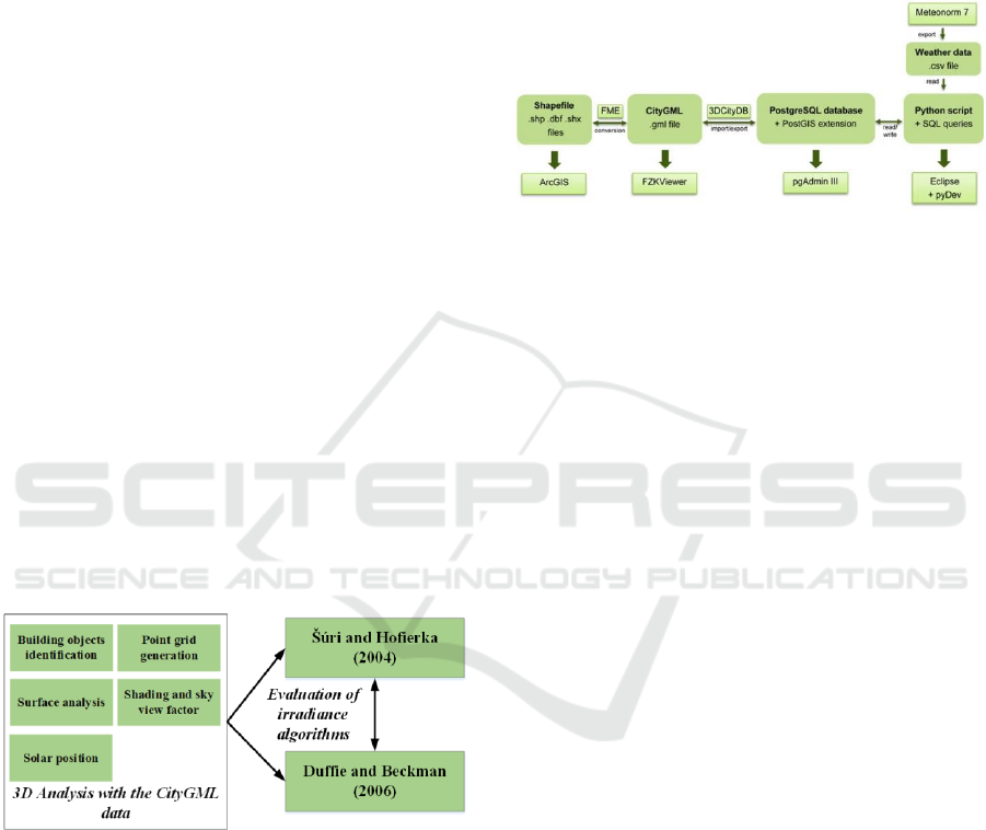
2.1 Main Approach

The broad methodological steps of this study can be

divided into 3 main parts (Figure 1). First, the

analyses of the 3D city models (e.g., CityGML

format) include preparation of the data, configuration

of the software and tools, generation of the point grids

on the building surface, calculation of the shading and

sky view factor of the points, solar position, etc.

(Section 3.1). Then the outcomes of these analyses

are considered as inputs to both solar irradiance

algorithms. The algorithm proposed by Šúri and

Hofierka (2004) was adapted earlier to calculate

monthly irradiation on CityGML data (Wieland et al.,

2015). This study improves the previous modelling

approach to incorporate the calculation of hourly

irradiance and advance the 3D analyses part. In this

regard, hourly measured weather data of a ground

station is considered (Section 3.2). Afterwards, the

algorithm proposed by Duffie and Beckman (2006) is

implemented, which also requires the same weather

data (Section 3.3). Both algorithms estimate solar

irradiance (direct and diffuse) on horizontal, vertical

and tilted surfaces on an hourly basis. In order to

perform a comparative evaluation of both algorithms,

the spatial and temporal irradiation results are

aggregated to buildings and annual level,

respectively. Finally, the results are visualized and

evaluated (Section 4).

Figure 1: Broad methodological approach.

2.2 Data

The hourly weather data on wind speed, temperature

and horizontal radiation are collected from the

Meteonorm software in TMY3 format (Wilcox and

Marion, 2008). The 3D city model of the CityGML

format having Level of Detail 2 (LoD2 includes

appropriate roof structure) of the city of Karlsruhe is

also gathered. A detailed description of the CityGML

data format and different LoDs is given in (OGC,

2012).

2.3 Software Architecture

Several software such as FME, 3DCityDB,

pgAdminIII and Eclipse are deployed to perform the

3D and solar irradiance analysis (Murshed et al.,

2017). The algorithms are written in Python scripts,

considering the object oriented approach (Figure 2).

Figure 2: Software architecture and data flow (Murshed et

al., 2017).

The LoD2 data of the CityGML format are

imported in a PostgreSQL database provided with

PostGIS extension, which allows treating spatial

objects by creating a special structure in the database.

The original CityGML file is adapted to the relational

schema by transforming through 3DCityDB, which

reorganizes files into specific tables. Finally, the data

can be retrieved using the Python code for further

calculations, analysis, and saving of results.

3 IMPLEMENTATION

3.1 3D Analysis Part

The 3D analysis part involves treating of CityGML

data and performing necessary geometric

calculations. The main steps are:

a. Surface analysis,

b. Definition of the objects: building, surface

and surface points,

c. Creation of the grid of surface points,

d. Shading characterization and sky view

factor calculation,

e. Solar position and characterization.

Figure 3 explains the different processing steps,

inputs and calculated results.

a. Surface analysis is the main module from which

all other 3D analysis parts are called. It determines

which points are “shared” i.e., in-between two

surfaces. This is done by spatial analysis and by

checking for an intersection of a buffer (0.1 m)

around the point, if any other wall surface is nearby.

Such an assumption helps to avoid unnecessary

Evaluation of Two Solar Radiation Algorithms on 3D City Models for Calculating Photovoltaic Potential

297

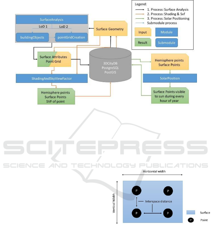
Figure 3: Detailed description of the inputs, different steps and associated results of the 3D analysis part. The outcome of the

analyses are saved in the PostgreSQL database.

spatial calculations, in case surface objects of

neighboring buildings may have geometric problems

(due to the bad quality of 3D city model).

b. The building object module identifies the wall,

roof or ground surfaces of the LoD2 (or LoD1) city

models. Then it performs different geometric

calculations such as normal vector, slope and aspect

of surface, using linear algebra.

c. The point grid module creates an homogenous

point grid on geometrical objects in 3D space (Figure

4). At first, considering the envelope of the geometry

(i.e., building surface), a starting point (3D point with

X,Y,Z) is defined. From this point, a distance is added

to the right (horizontal) as long as the sum of

interspaces (distance among points) is below the

expansion value X. Afterwards, the same procedure

is performed for all points as a step up (vertical) as

long as the interspace distance is below the expansion

value Y. Then the newly created points are checked,

if they are inside the polygon. This check is done once

per surface after the point distribution. Points outside

of the polygon are deleted. This approach is applied

for the horizontal polygons/surfaces. For non-

horizontal surfaces, points are rotated around the

axes, according to the orientation of the

corresponding polygon.

Therefore, technically speaking, the point grid

distribution is performed in 4 ways, depending on the

LoDs of the surface and the type of surface (e.g.,

ground, wall or roof surface). For LoD1, two

methods, one for horizontally orientated surfaces and

the other for vertically orientated surfaces are

observed. For LoD2, the points for horizontal

surfaces are distributed with the same method as

LoD1. For vertical surfaces, each point is rotated with

a matrix calculation into the plane of the surface

orientation. For tilted surfaces, different height values

of the geometry are taken into account to perform

point distribution.

Figure 4: Point grid creation on the surface.

d. Shading is performed through spatial analysis.

From each surface point, a line is created towards a

point of the hemisphere (a hemisphere of points is

created according to the horizontal and vertical

intervals chosen earlier, see Figure 5). If the line

intersects with another object (e.g., surface of the

same building, or another building) the surface point

is considered as shaded. If the line is not intersected

with another object, the corresponding surface point

is considered as not shaded. This process is done for

GISTAM 2018 - 4th International Conference on Geographical Information Systems Theory, Applications and Management

298

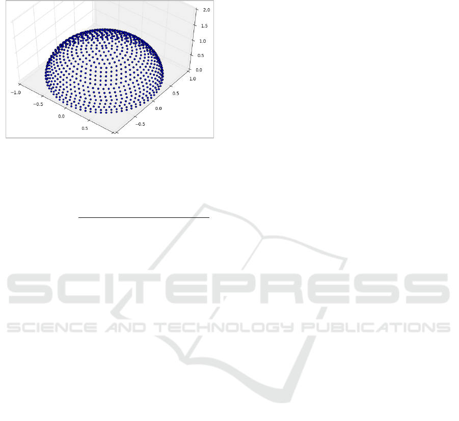
each surface point for every hemisphere direction

separately.

Figure 5: Hemisphere represented by sample points.

The sky view factor for each point is calculated as

the ratio between the number of visible hemisphere

points and the total number of hemisphere points.

𝑠𝑘𝑦 𝑣𝑖𝑒𝑤 𝑓𝑎𝑐𝑡𝑜𝑟 =

𝑛𝑢𝑚𝑏𝑒𝑟 𝑜𝑓 𝑣𝑖𝑠𝑖𝑏𝑙𝑒 ℎ𝑒𝑚𝑖𝑠ℎ𝑒𝑟𝑒 𝑝𝑜𝑖𝑛𝑡𝑠

𝑡𝑜𝑡𝑎𝑙 𝑛𝑢𝑚𝑏𝑒𝑟 𝑜𝑓 ℎ𝑒𝑚𝑖𝑠ℎ𝑒𝑟𝑒 𝑝𝑜𝑖𝑛𝑡𝑠

e. Finally, solar position is calculated. For each

surface point, the IDs of the hemisphere directions,

which are visible, are stored in an array. To detect

whether a surface point is shaded at a certain time, the

position of the sun is computed for a specific time of

the day and the closest hemisphere direction is

determined. If the ID of this hemisphere direction is

contained in the array of the surface point, the point

is considered not to be shaded at that time of the day.

For each surface point this is performed 8760 times,

which corresponds to the number of hours per year.

The information of whether a surface point is shaded

at a certain hour is stored as a Boolean value, either

“True = is shaded” or “False = is not shaded”.

3.2 Solar Irradiance Algorithm by Šúri

and Hofierka (2004)

This algorithm is applied in many studies and an open

source GIS environment is employed. Computation is

quick and local meteorological data can be adapted to

the model. It is robust, and requires few input

parameters (Gueymard, 2012).

The process of computing solar irradiance (clear

sky) begins with the determination of the

extraterrestrial irradiance, which varies during the

year. After the position of the sun is calculated with

respect to time, the day and the latitude of the location

of interest, the beam and diffuse component of solar

irradiance on a horizontal surface can be determined

for the time of interest with respect to the Linke

turbidity. By incorporating the slope and the surface,

the incidence angle of solar rays on this surface can

be computed. With this angle, the horizontal radiation

components are adjusted according to the orientation

of the surface (Šúri and Hofierka, 2004). In this

model, only shadowing of the beam component is

taken into account, and not of the diffuse irradiance.

3.3 Solar Irradiance Algorithm by

Duffie and Beckman (2006)

It is calculated in four main steps. At first, the sun

position is calculated depending on the location

coordinates and time. Then the direct normal

irradiance is calculated considering the sinus of the

solar elevation angle, global horizontal and diffuse

horizontal irradiances that can be found in the

weather data. Then, based on the sun position vector

and the normal vector to the surface, the incidence

angle of the beam irradiance is computed and the

shadowing of the beam irradiance is included as

calculated previously. The sky view factor is applied

to diffuse irradiance.

Afterwards, an anisotropic sky model, known as

the Hay-Davies-Klucher-Reindl model is used to take

into account circumsolar diffuse irradiance and

horizon-brightening (Duffie and Beckman, 2006).

Finally, hourly direct and diffuse radiation are

calculated.

3.4 Assumptions

Both algorithms calculate only direct and diffuse

solar radiation. In order to have a comparative

evaluation, all relevant parameters are considered

identical. About 96 hemisphere points were created to

determine the sky view factor and to identify if each

surface is visible to particular hemisphere points (and

to solar position) throughout each hour of a year. A

point grid of 5m resolution is created on the building

surfaces. The measured weather data of a weather

station are used as inputs to both algorithms.

4 VISUALIZATION AND

DISCUSSION OF RESULTS

In order to perform a quick comparative evaluation of

the irradiance results, both algorithms were run on 95

buildings (having 650 surfaces) in a neighborhood in

the City of Karlsruhe in Germany. Then in order to

test the applicability of the implemented model, we

ran it for about 12000 LoD2 buildings in another

district of the same city.

Evaluation of Two Solar Radiation Algorithms on 3D City Models for Calculating Photovoltaic Potential

299

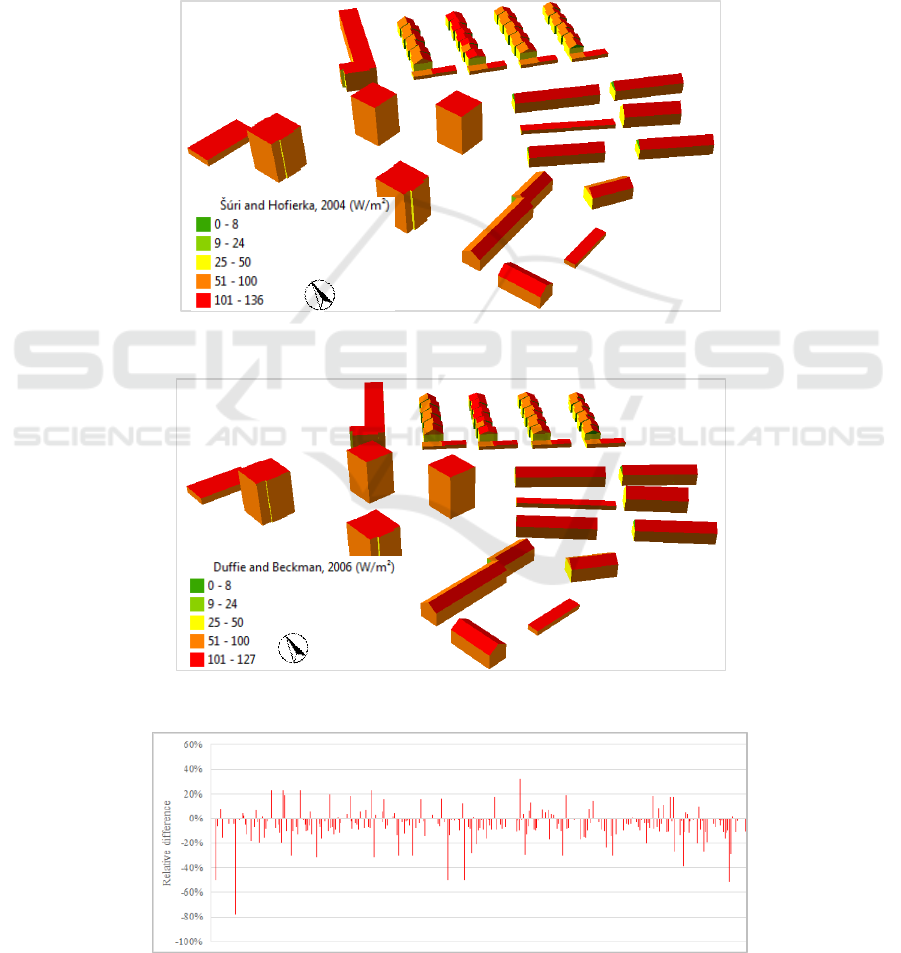
The direct and diffuse radiation were first

calculated for each point on the building surface,

which were then aggregated for each surface to

display the hourly averaged irradiance throughout the

year (W/m²). In analyzing the results of the first

method, we found the minimum and maximum values

to be 25 and 136 W/m² (Figure 6), whereas in the

second method, the values were 8 and 127 W/m²

(Figure 7), respectively.

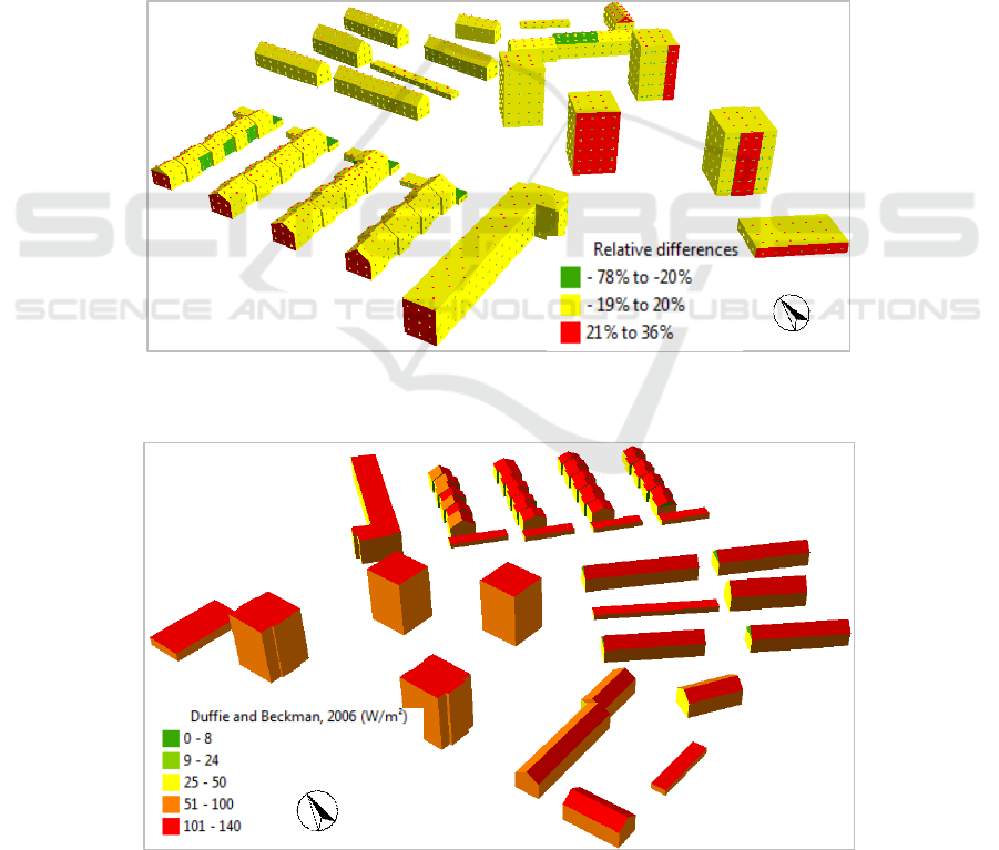
Some surfaces displayed exactly the same results

for both algorithms. We observe that the initial

method estimates higher solar irradiances (up to 78%)

on the surfaces that are partially shaded by

neighboring surfaces (Figure 8).

We also observe that both algorithms calculate

almost the same solar irradiance on the roof surfaces.

It is found out that the second algorithm calculates

slightly higher solar irradiances (up to 36%) on the

north oriented surfaces (Figure 9).

It is evident that tilted surfaces (directing towards

the sun) will receive more irradiance than flat

surfaces. In case of flat roofs (e.g., where slope is

Figure 6: Hourly average solar irradiation on horizontal and vertical surfaces after Šúri and Hofierka (2004).

Figure 7: Hourly average solar irradiation on horizontal and vertical surfaces after Duffie and Beckman (2006).

Figure 8: Relative difference of irradiance results on some surfaces detected by the two algorithms.

GISTAM 2018 - 4th International Conference on Geographical Information Systems Theory, Applications and Management

300

<20°), the PV installations are normally optimized by

tilting the panels so that they can receive maximum

solar radiation and thus can optimize energy

production for the PV panels. Therefore, the

calculation of irradiance on such tilted surfaces

(analogous to the PV installation surfaces) is very

important. The second method can be adapted to

calculate radiation on such surfaces. For example, we

found that the irradiance on a tilted surface is 140

W/m², which is higher than the radiation calculated

earlier on the actual roof surface (127 W/m²), which

has a slope less than <20° (Figure 10).

Both models were run on the same virtual

machine with standard configurations. The run time

of both models with 95 buildings was almost the same

(approximately 4 minutes). The multi-processing

functions of python helped to improve the model run

time.

Based on the results, it is difficult to justify which

method is more accurate and suitable for PV potential

analyses, although both of them considered similar

input datasets and assumptions. Nevertheless,

observing the evidence that the method by Duffie and

Beckman (2006) performs more realistic calculations

for the surfaces which are next to shaded surfaces

(confirmed after site inspection) and the flexibility of

assessing the irradiance on tilted surfaces, this

method is more suitable for photovoltaic assessment

in urban areas. Therefore, the algorithm proposed by

Duffie and Beckman (2006) was applied to around

12000 LoD2 buildings (consisting of approximately

96000 surfaces and 442000 points) in the city of

Karlsruhe in Germany to calculate hourly irradiance

on the tilted and vertical surfaces. It took

approximately 7 hours to complete the analysis.

Figure 9: Relative difference in solar irradiance on the wall and roof surfaces observed by the two methods. The grid points

are displayed on the surface on which solar radiation is calculated first.

Figure 10: Hourly average solar irradiation over a year on tilted surfaces (where slope was <20°) after Duffie and Beckman

(2006).

Evaluation of Two Solar Radiation Algorithms on 3D City Models for Calculating Photovoltaic Potential

301

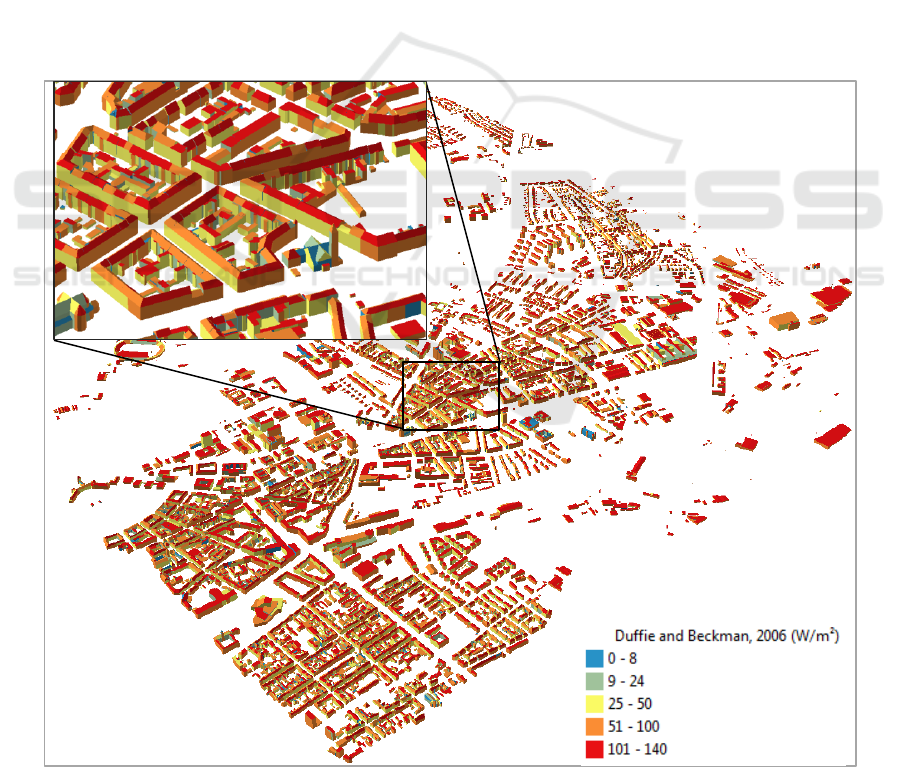
Figure 11 illustrates the hourly average solar

irradiance over a year on the vertical and tilted

surfaces of the buildings. The surfaces that strike out

in red are those that have few neighbouring buildings

obstructing sunlight. Generally, these are tilted

rooftops and this visualization quickly identifies the

best sun exposure.

5 CONCLUSIONS

Two solar irradiation algorithms were tested in this

study to perform a comparative evaluation of

irradiation results with a view to assess PV potential

in a city or district. For this reason, CityGML data and

an open source software infrastructure was used to

perform a quick but robust calculation of direct and

diffuse radiation of different building surfaces.

Moreover, with the semantic relationship among the

points, surfaces and buildings within the CityGML

data, it was possible to aggregate the results on

different spatial and/or temporal (hourly, monthly,

yearly, etc.) resolutions. The testing of the model with

about 12000 LoD2 buildings in the city of Karlsruhe

showed the applicability of these algorithms at a city

scale.

Several limitations are also evident in this study.

For instance, reflected radiation was not calculated. It

can be added by calculating the ground view factor.

Increasing the number of hemisphere points will

improve the model accuracy but will also increase the

run time. Therefore, in the future, the results can be

tested with a varying number of hemisphere points

and grid points. Consideration of shading due to

vegetation or chimneys will also improve the

calculation of solar irradiance.

As a continuation of this study, considering the

amount of solar radiation received by the sun, the PV

potential in terms of electrical energy (kWh),

investment costs (Euro) and levelized cost of energy

(LCOE) on the horizontal, vertical and tilted surfaces

will be calculated. The results can be integrated into

Figure 11: Hourly average solar irradiation (W/m²) over a year on tilted (where slope was <20°) and vertical surfaces after

Duffie and Beckman (2006) on 12000 LoD2 buildings in Karlsruhe, Germany.

GISTAM 2018 - 4th International Conference on Geographical Information Systems Theory, Applications and Management

302

a web platform, in order to visualize in 3D and to

allow the decision makers and citizens to ascertain the

solar irradiance and techno-economic PV potentials

in a flexible manner.

ACKNOWLEDGEMENTS

We would like to thank City of Karlsruhe for the

permission of using CityGML data and the project

“Smart and Low Carbon Cities” of EDF R&D for

funding the research. We are also grateful to Manfred

Wieland for his initial contribution in coding and the

three anonymous reviewers for their constructive

comments on our manuscript.

REFERENCES

Bahu, J.-M., Koch, A., Kremers, E. & Murshed, S. M. 2014.

Towards a 3D spatial urban energy modelling

approach. International Journal of 3-D Information

Modeling (IJ3DIM), 3, 1-16.

Catita, C., Redweik, P., Pereira, J. & Brito, M. C. 2014.

Extending solar potential analysis in buildings to

vertical facades. Computers & Geosciences, 66, 1-12.

Duffie, J. A. & Beckman, W. A. 2006. Solar engineering of

thermal processes, Wiley New York.

Freitas, S., Catita, C., Redweik, P. & Brito, M. 2015.

Modelling solar potential in the urban environment:

State-of-the-art review. Renewable and Sustainable

Energy Reviews, 41, 915-931.

Gueymard, C. A. 2012. Clear-sky irradiance predictions for

solar resource mapping and large-scale applications:

Improved validation methodology and detailed

performance analysis of 18 broadband radiative

models. Solar Energy, 86, 2145-2169.

Hachem, C., Fazio, P. & Athienitis, A. 2013. Solar

optimized residential neighborhoods: Evaluation and

design methodology. Solar Energy, 95, 42-64.

Huld, T. 2017. PVMAPS: Software tools and data for the

estimation of solar radiation and photovoltaic module

performance over large geographical areas. Solar

Energy, 142, 171-181.

Lee, J. & Zlatanova, S. 2009. Solar radiation over the urban

texture: LIDAR data and image processing techniques

for environmental analysis at city scale. In: LEE, J. &

ZLATANOVA, S. (eds.) 3D Geo-Information

Sciences, Lecture Notes in Geoinformation and

Cartography. Berlin, Heidelberg: Springer.

Li, Y. & Liu, C. 2017. Estimating solar energy potentials

on pitched roofs. Energy and Buildings, 139, 101-107.

Murshed, S. M., Picard, S. & Koch, A. 2017. CityBEM: An

Open Source Implementation and Validation of

Monthly Heating and Cooling Energy Needs for 3D

Buildings in Cities. ISPRS Ann. Photogramm. Remote

Sens. Spatial Inf. Sci., IV-4/W5, 83-90.

Nguyen, H. & Pearce, J. M. 2010. Estimating potential

photovoltaic yield with r. sun and the open source

geographical resources analysis support system. Solar

energy, 84, 831-843.

Ogc 2012. OGC City Geography Markup Language

(CityGML) Encoding Standard 2.0.0. Open Geospatial

Consortium.

Redweik, P., Catita, C. & Brito, M. 2013. Solar energy

potential on roofs and facades in an urban landscape.

Solar Energy, 97, 332-341.

Šúri, M. & Hofierka, J. 2004. A new GIS‐based solar

radiation model and its application to photovoltaic

assessments. Transactions in GIS, 8, 175-190.

Vitucci, E. M., Falaschi, F. & Degli-Esposti, V. 2014. Ray

tracing algorithm for accurate solar irradiance

prediction in urban areas. Applied optics, 53, 5465-

5476.

Wieland, M., Nichersu, A., Murshed, S. M. & Wendel, J.

2015. Computing Solar Radiation on CityGML

Building Data. 18th AGILE International Conference

on Geographic Information Science. June 9 - 12, 2015,

Lisbon.

Wilcox, S. & Marion, W. 2008. Users manual for TMY3

data sets. Colorado: National Renewable Energy

Laboratory (NREL).

Evaluation of Two Solar Radiation Algorithms on 3D City Models for Calculating Photovoltaic Potential

303