
Hierarchical Electricity Demand Forecasting by Exploring the
Electricity Consumption Patterns
Yue Pang
1
, Chaoyi Jin
1
, Xiangdong Zhou
1
, Naiwang Guo
2
and Yong Zhang
2
1
School of Computer Science, Fudan University, Shanghai, China
2
State Grid Shanghai Municipal Electric Power Company, Shanghai, China
Keywords: Hierarchical Forecasting, Aggregate Constraints, Consumption Pattern.
Abstract: Accurate electricity demand forecasting is necessary to develop an efficient and sustainable power system.
Total demand of the whole region can be disaggregated at different levels, thus producing a hierarchical
structure. In the hierarchical demand forecasting, the prediction accuracy and aggregate consistency between
levels are two important issues, however in the previous works the prediction accuracy is often affected by
conducting the aggregate consistency. In this work, we propose a novel pattern-based hierarchical time series
forecasting (PHF) method which consists of two aggregation stages. In the first aggregation stage, by
exploring the electricity consuming patterns with clustering method, the bottom level electricity demand
forecasting is improved, and in the second stage the region level aggregation is conducted to achieve the
whole level forecasting. The experiments are conducted on the Energy Demand Research Project (EDRP)
datasets, and the experimental results show that compared with the previous state-of-the-art methods, our
method improves the prediction accuracy in all hierarchical levels with keeping aggregation consistency.
1 INTRODUCTION
Due to the existing problem of inconvenience
electricity storage, excess electricity would cause
unnecessary waste. Accurate forecasting is helpful to
guide the electric power companies to make decision.
Thus, electricity demand forecasting is one of the
most important problems in the field of electric power
management. With the rapid growth of smart grid,
more and more meter data are becoming available,
which brings potential of improving the prediction of
the power demand with more delicacy.
Recently, hierarchical electricity demand
forecasting attracts more and more research attentions
(Taieb et al., 2017). Total consumption in the whole
geographic region can be geographically
disaggregated into several sub-regions, and these sub-
regions can be further disaggregated into regions at
lower level. For example, electricity consumption in
countries can be disaggregated into provinces, cities,
districts, etc. That is, electricity time series can be
represented in a hierarchical structure. From top
down, the structure contains series at top level, high
level, low level and bottom level. According to the
above geographic disaggregate strategy, the time
series in different levels must obey the aggregation
constraints, i.e. the demand in different levels should
be summed consistently. Most of the state-of-the-art
hierarchical predication methods estimate initial
forecasts and then reconcile them to ensure aggregate
constraints. However, it is noticed that the regional
aggregation consistency cannot improve the whole
level prediction accuracy (Hyndman et al., 2011).
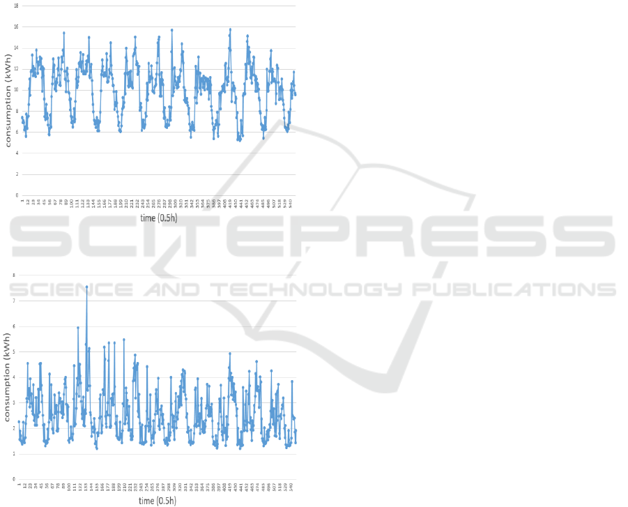
The electricity consuming pattern can be found by
clustering analysis on the time series of electricity
usage with the similarity measurements. Figure 1
illustrates the aggregation time series of electricity
consumption by clustering and random selection. We
notice that in this Figure the aggregated time series
obtained by clustering of similar time series shows
more stable and regular than the series aggregated by
randomly selected ones. The experience and some
previous work (Wijaya et al., 2015) show that the
stable and regular time series are very good (or ideal)
for prediction or regression. Therefore, we are
motivated to exploit the time series clustering to
improve the bottom level electricity demand
prediction and manage to improve the regional
hierarchal predication accuracy.
In this paper we propose a novel pattern-based
hierarchical demand forecasting (PHF) method which
consists of two aggregation stages. The proposed
576
Pang, Y., Jin, C., Zhou, X., Guo, N. and Zhang, Y.
Hierarchical Electricity Demand Forecasting by Exploring the Electricity Consumption Patterns.
DOI: 10.5220/0006715005760581
In Proceedings of the 7th International Conference on Pattern Recognition Applications and Methods (ICPRAM 2018), pages 576-581
ISBN: 978-989-758-276-9
Copyright © 2018 by SCITEPRESS – Science and Technology Publications, Lda. All rights reserved
method improves the whole level regional demand
prediction accuracy by exploring the electricity
consuming clustering and the aggregation
consistency. Specifically, at the first aggregation
stage, the proposed method constructs a hierarchical
structure based on electricity consuming pattern by
clustering analysis. Then, the bottom-level series are
then reconciled appropriately through the aggregation
constraints in the hierarchy. At the second
aggregation stage, we aggregate the refined
individual predication to improve the regional
demand prediction.
(a) The aggregated series of electricity consumption of 7
households by time series clustering.
(b) The aggregated electricity consumption of 7 random
selected individual households.
Figure 1: Aggregated electricity consumption series by
clustering and random selected households on real datasets.
To our best knowledge, this is the first work of
forecasting hierarchical regional electricity demand
by using electricity consumption pattern analysis. The
experiments are conducted by using real electricity
dataset. The experimental results demonstrate that our
proposed method not only satisfies consistency
relationship between different levels, but also
improves the prediction accuracy in all regional levels.
Compared with the previous methods, our method
achieves 0.07 and 0.03 lower prediction error in the
evaluation measurements of Mean Absolute
percentage Error (MAPE) and Mean Square Error
(MSE) respectively.
2 RELATED WORK
The related works of forecasting demand in
hierarchical structure mainly include classical
forecasting and optimal combined forecasting.
2.1 Classical Forecasting
Classical forecasting is also called base forecasting
(BASE) (Hyndman et al., 2011). It forecasts time
series in all levels independently. The common
forecasting models used in BASE forecasting are:
Exponential Smoothing State Space (ETS),
Autoregressive Integrated Moving Average (ARIMA)
and ETS with Box-Cox Transformation, ARMA
Errors, Trend and Seasonal Components (TBATS)
(De Livera et al., 2011). The merit of BASE is that
forecasts in different levels do not influence each
other, resulting in high prediction accuracy at all
levels. But the shortcoming is that the forecasts
usually do not satisfy the aggregation consistency.
2.2 Optimal Combined Forecasting
Optimal combined forecasting (OPT) method firstly
obtains initial forecasts in all levels using BASE
(Hyndman et al., 2011). According to the aggregation
constraints, optimal combined forecasts are then
obtained by revising series in all levels. The key
process of OPT is to estimate covariance matrix of
forecast error. Two common methods of estimating
covariance matrix are optimal combined forecasting
based on ordinary least square and weight least square
(OPT-OLS and OPT-WLS). Owing to the revision,
OPT has the advantage of satisfying aggregate
constraints over BASE. However the excess revising
may affect the overall prediction accuracy.
(1) OPT-OLS
In 2011, Hyndman et al. estimates covariance
matrix using ordinary least square (Hyndman et al.,
2011). Optimal-OLS assumes that covariance matrix
can be equivalent to a coefficient matrix multiple
identify matrix.
Hierarchical Electricity Demand Forecasting by Exploring the Electricity Consumption Patterns
577
(2) OPT-WLS
In 2016, Hyndman et al. estimates covariance
matrix using weight least square (Hyndman et al.,
2016). Optimal-WLS assumes that covariance matrix
can be equivalent to a coefficient matrix multiple
diagonal matrix. The diagonal matrix is constructed
using sample variance of BASE forecasts errors.
3 PATTERN-BASED
HIERARCHICAL TIME SERIES
FORECASTING
Electricity time series can represent the consumption
behaviour of residential user, namely electricity
consumption pattern. Compared to time series
aggregated by randomly selected, consumption
pattern obtained by clustering of similar ones shows
more stable and regular, hence reduces the difficulty
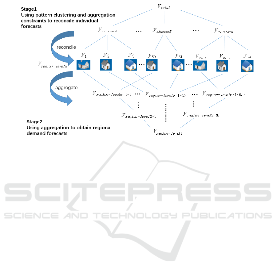
of series prediction. A novel pattern-based
hierarchical time series forecasting (PHF) is proposed
in the paper. The idea is illustrated in Figure 2.
For convenience, we define some symbols. n
denotes the number of series at all levels.
denotes
an n-length vector with observations at time t and all
levels.
denotes the number of series at bottom
level.
denotes an n
b
-length vector with
observations at time t and bottom levels. S denotes an
summing matrix constructed from the
hierarchical structure. According to hierarchical
structure constructed from geographic data, these
symbols can be associated through equation (1)
(Taieb et al., 2017).
(1)
PHF mainly includes two stages of aggregations,
the specific procedures are as follows.
(1) Stage 1
Electricity consumption patterns of all individual
time series are extracted by k-means clustering. The
process of k-means clustering can be defined with
equation (2) (Hartigan and Wong, 1979).
(2)
where
is the mean of all points in cluster
.
According to the results of clustering, hierarchical
structure based on electricity consumption pattern
and the corresponding summing matrix
are
obtained.
We let
be an n-length vector of h-step ahead
initial forecasts estimated with historical observations
at time t and all levels.
,
,
.
is obtained by BASE.
And we use classical models to forecast series. For
example, equation (3) is the forecast equation of
simple exponential smoothing model (Hyndman et al.,
2002).
Figure 2: The strategy of PHF.
ICPRAM 2018 - 7th International Conference on Pattern Recognition Applications and Methods
578

(3)
where is smoothing parameter, .
is
the first forecast value of
.
In order to improve the predication accuracy of
bottom level series, we reconcile initial forecasts at
bottom level according to the higher level cluster
aggregation predication. The bottom revised forecasts
can be estimated by solving the following regression
as shown in equation (4) (Hyndman et al., 2011).
(4)
where
is the mean of forecasts at bottom level.
is the reconciled error, whose mean and variance
is zero and covariance matrix
.
(5)
where
and
are real and estimated value of
h-step ahead forecasts with historical observations at
time T separately.
We estimate
by MinT (Wickramasuriya et
al., 2015). Its main idea is to minimize the trace of
variance of forecast errors by equation (6).
(6)
where
denotes the transpose of
.
(2) Stage 2
According to the geographic data, geography-
based hierarchical structure and corresponding
regional summing matrix
are obtained. Here, we
assume the hierarchy contains m levels, and
indicates the number of series in levels m-1. Based on
estimated bottom-level forecasts obtained at stage 1,
the region demand forecasts
are obtained
according to equation (7).
(7)
So far , we obtain the final results
.
4 EXPERIMENTS
4.1 Data
We use the public datasets from Energy Demand
Research Project: Early Smart Meter Trials (EDRP),
which is conducted by four energy suppliers in
England (AECOM, 2011). EDRP datasets contains
about 14000 electricity consumption of residential
consumers during January, 2009 and September,
2010. The electricity consumed is measured during
half-hour interval. We extract 2501 smart meters with
data available between May 9th, 2009 and August
24th, 2009.
We obtain the information of regional division-
based hierarchical structure from geographic data.
The hierarchy contains six levels. The numbers of
series at different level are: 1 (level 1), 7 (level 2), 12
(level 3), 21 (level 4), 44 (level 5) and 2501 (level 6).
4.2 Experimental Setup
We use data at the time interval from 1 to T as
historical data to predict data at time T+h, where T
ranges from 500 to 549 and h=1. In one experiment,
we conduct 50 forecasting tasks and compute mean
forecast accuracy for all tasks.
We compare PHF with the methods introduced in
the related work (Section 2 in the paper). In PHF, the
eight types of pattern are extracted by k-means
clustering at the first aggregation stage. In
comparison method, we choose BASE, OPT-OLS
and OPT-WLS. In all the experiments, we use ETS,
ARIMA and TBATS as the basic models of
independent forecasting respectively.
4.3 Evaluation Metrics
In the experiment, we use Mean Absolute Percentage
Error (MAPE) and Mean Square Error (MSE) as the
metrics for evaluating.
(1) MAPE
The definition of MAPE is (Wijaya et al., 2015):
(8)
where
and
are real and estimated value of
forecasts at time t respectively, n indicates the number
of series in all levels. First, compute the MAPE
measurement of forecast error in every forecasting
task. Second, compute average value of 50 tasks as
the final evaluation measurement. When MAPE
Hierarchical Electricity Demand Forecasting by Exploring the Electricity Consumption Patterns
579

measurement is lower, the method has higher
prediction accuracy.
(2) MSE
The definition of MSE is (Yang et al., 2017):
(9)
The procedure of computing the MSE measurement
is similar to that of MAPE. Likewise, the method has
higher prediction accuracy when its MSE
measurement is lower.
4.4 Experimental Results
According to the experimental results of aggregate
consistency, both OPT and PHF do satisfy the
geographic aggregate constraints, but BASE does not.
In term of prediction accuracy, the experimental
results are shown in following tables.
Table 1: The comparison of prediction accuracy by methods
based on ETS (all levels).
Method
MAPE
MSE
BASE-ETS
0.68
1.02
OPT-OLS-ETS
0.69
1.01
OPT-WLS-ETS
0.64
1.02
PHF-OLS-ETS
0.64
0.90
PHF-WLS-ETS
0.64
0.92
In first experiment, we use ETS model to forecast
time series. The results are shown in Table 1. Under
the measurement of MAPE, PHF (0.64) has higher
prediction accuracy than BASE (0.68), while OPT-
OLS (0.69) has lower prediction accuracy than BASE
(0.68). This indicates that OPT-OLS meets aggregate
consistency at cost of prediction accuracy. In contrast,
PHF can improve overall prediction accuracy, as well
as satisfy aggregation constraints. Under the
measurement of MSE, although OPT-OLS (1.01)
enhances predicting ability of BASE (1.02), PHF
(0.90) has stronger predicting ability. It also means
that PHF has higher forecasting accuracy on the
premise of meeting aggregate constraints. In term of
weight least square estimation, we come to the same
conclusion. PHF-OLS-ETS has the highest prediction
accuracy in consideration of both MAPE and MSE
measurement.
Table 2: The comparison of prediction accuracy by methods
based on ETS (bottom levels).
Method
MAPE
MSE
BASE-ETS
0.69
0.06
OPT-OLS-ETS
0.69
0.06
OPT-WLS-ETS
0.66
0.06
PHF-OLS-ETS
0.66
0.06
PHF-WLS-ETS
0.65
0.06
The forecasting accuracy for 2501 time series at
bottom level using ETS model is shown in Table 2.
Under the measurement of MAPE, PHF-OLS-ETS
(0.66) achieves highest prediction accuracy,
compared with OPT-OLS-ETS (0.69) and BASE-
ETS (0.69). Under the measurement of MSE, all
methods achieve the same prediction accuracy. It is
because the values of bottom forecasts are very small,
MSE is not enough for measuring the difference
between methods. In consideration of both MAPE
and MSE measurement, PHF-WLS-ETS achieves the
best prediction accuracy. This demonstrates that PHF
appropriately reconciles the series at bottom level
through aggregation constrains at the first stage 1.
According to Table 1, the region forecasts by PHF
have less errors compared to OPT. This is because
that regional forecasts of series at all levels are
computed through aggregation constraints based on
the improved forecasts of bottom series.
In the next experiment, we use ARIMA model to
forecast time series. The results are shown in Table 3.
Table 3: The comparison of prediction accuracy by methods
based on ARIMA (all levels).
Method
MAPE
MSE
BASE-ARIMA
0.70
0.95
OPT-OLS-ARIMA
0.74
0.92
OPT-WLS-ARIMA
0.65
0.95
PHF-OLS-ARIMA
0.67
0.89
PHF-WLS-ARIMA
0.65
0.93
Similar to the above analysis, PHF (MAPE:
0.67/0.65, MSE: 0.89/0.93) achieves higher
forecasting accuracy than OPT (MAPE: 0.74/0.65,
MSE: 0.92/0.95) when using OLS or WLS.
Especially, the MAPE measurement of forecasts
obtained by PHF is 0.07 less than OPT, and the MSE
measurement of forecasts obtained by ECPHF is 0.03
less than OPT.
In the last experiment, we replace ARIMA with
TBATS model. The results are shown in Table 4.
PHF-TBATS (MAPE: 0.62/0.62, MSE: 0.93/0.95)
still forecasts more accurately than OPT-TBATS
(MAPE: 0.73/0.62, MSE: 0.97/0.95).
ICPRAM 2018 - 7th International Conference on Pattern Recognition Applications and Methods
580

Table 4: The comparison of prediction accuracy by methods
based on TBATS (all levels).
Method
MAPE
MSE
BASE-TBATS
0.45
1.00
OPT-OLS-TBATS
0.73
0.97
OPT-WLS- TBATS
0.62
0.95
PHF-OLS- TBATS
0.62
0.93
PHF-WLS- TBATS
0.62
0.95
In conclusion, compared with the previous
methods, our method achieves the best prediction
accuracy on average of all the 2586 series in the
hierarchy with keeping aggregation consistency.
5 CONCLUSIONS
We focus on hierarchical demand forecasting in the
paper. Both the high prediction accuracy and
aggregate consistency should be considered in the
forecasting. However, in order to keep the aggregate
consistency, prediction accuracy is usually affected
(reduced) in the previous works. To deal with the
problem, we propose a novel hierarchical demand
forecasting method based on electricity consumption
pattern analysis with a two stage algorithm. It
reconciles forecasts of bottom series at first
aggregation stage and further improves regional
demand forecasts at second aggregation stage. The
experimental results based on the Energy Demand
Research Project datasets demonstrate that compared
with the previous state-of-the-art methods, our
method achieves the best forecasting accuracy while
keeping aggregation consistency.
ACKNOWLEDGEMENTS
This work was supported by the National High
Technology Research and Development Program
(863 Program) of China (2015AA050203) and NSFC
grant no. 61370157.
REFERENCES
Taieb, S. B., Yu, J., Barreto, M. N., Rajagopal, R., 2017.
Regularization in Hierarchical Time Series Forecasting
with Application to Electricity Smart Meter Data. In
AAAI, 31th AAAI Conference on Artificial
Intelligence. 4474-4480.
Hyndman, R. J., Ahmed, R. A., Athanasopoulos, G.,
Shang, H. L., 2011. Optimal combination forecasts for
hierarchical time series. Computational Statistics and
Data Analysis. 55(9), 2579-2589.
Wijaya, T. K., Vasirani, M., Humeau, S., Aberer, K., 2015.
Cluster-based aggregate forecasting for residential
electricity demand using smart meter data. In 2015
IEEE International Conference on Big Data. 879-887.
De Livera, A. M., Hyndman, R. J., Snyder, R. D., 2011.
Forecasting time series with complex seasonal patterns
using exponential smoothing. Journal of the American
Statistical Association. 106(496), 1513-1527.
Hyndman, R. J., Lee, A. J., Wang, E., 2016. Fast
computation of reconciled forecasts for hierarchical and
grouped time series. Computational Statistics and Data
Analysis. 97, 16-32.
Hartigan, J. A., Wong, M. A., 1979. Algorithm AS 136: A
k-means clustering algorithm. Journal of the Royal
Statistical Society. Series C (Applied Statistics). 28(1),
100-108.
Hyndman, R. J., Koehler, A. B., Snyder, R. D., Grose, S.,
2002. A state space framework for automatic
forecasting using exponential smoothing methods.
International Journal of Forecasting. 18(3), 439-454.
Wickramasuriya, S. L., Athanasopoulos, G., Hyndman, R.
J., 2015. Forecasting hierarchical and grouped time
series through trace minimization. Department of
Econometrics and Business Statistics, Monash
University.
AECOM. 2011. Energy demand research project: Final
analysis. Technical report, AECOM House,
Hertfordshire, UK.
Yang, D., Quan, H., Disfani, V. R., Liu, L., 2017.
Reconciling solar forecasts: Geographical hierarchy.
Solar Energy. 146, 276-286.
Hierarchical Electricity Demand Forecasting by Exploring the Electricity Consumption Patterns
581
