Reducing Empty Truck Trips in Long Distance Network by Combining

Trips

arbara da Costa Rodrigues and Andr

e Gustavo dos Santos

Departamento de Inform

atica, Universidade Federal de Vic¸osa, Av. P. H. Rolfs s/n - 36570-900 Vic¸osa, MG, Brazil

Keywords:

Trips Combination, MILP, Heuristic, Combinatorial Optimization.

Abstract:

Brazilian import and export activities on ports are subject to considerable slow queues and congestion, revea-

ling a lack of medium and/or short-term logistic planning. One of the causes is the number of trucks traveling

with empty containers, performing one-way trips, from inland cities to the port or from the port to the cities.

This issue may be reduced by combining trips, i.e., after bringing goods to the port (export trip), a truck should,

when possible, carry goods from the port to the origin or a nearby city (import trip). In this paper we inves-

tigate a combinatorial optimization problem where a set of import/export/inland trips should be combined in

order to reduce total traveling time, which in turn reduces the number of empty trucks traveling to/from the

port. Individual trips and combined trips must obey national law regulation of resting time, as typical road trips

in Brazil covers hundreds, even thousands of kilometers. We also consider opening operation hours on each

location (time windows), which may force a driver to wait upon arriving. We test exact and heuristic appro-

aches, and present the total travel time and number of trucks needed for each solution, considering instances

based on real freight data.

1 INTRODUCTION

Due to the lack of infrastructure for grain storage,

most of the Brazilian production is destined to expor-

tation, leading to a high demand of freightage to the

ports, as well as import of fertilizers and other agri-

cultural inputs to the grain exporting regions (Cai-

xeta Filho, 2010). Most of the freight transport is

done by road modal, which may bring practicality,

agility and ﬂexibility in cases of route exchanges. Ne-

vertheless, a number of disadvantages may be listed,

for example, high cost of fuel and tolls, poor condition

of roads in some regions, among others. Those dis-

advantages, allied to lack of good logistic planning,

cause an extra cost to the ﬁnal price of the transpor-

ted goods, congestion in the port area, delivery delays

and also empty trucks, traveling without any freight.

Empty truck trips may be found specially on im-

port/export trips, when the carrier take care only of

incoming or outgoing trips. The result is a somehow

needless increasing in the number of trucks using the

roads and ports, consequently increasing congestion

and polluting gas emission generated by fuel combus-

tion (Schulte et al., 2015).

In the context of this work we have import trips, as

shown in Figure 1. The truck collects a freight (con-

tainer, bagged or bulk goods) at the port. Then travels

to a customer or depot that demands that freight. After

unloading, the truck travels back to the port unladen.

Figure 1: Import scenario.

An empty truck travel also occurs in export trips,

as shown in Figure 2. The truck collects goods at a

customer or a depot and travels to the port, where

sometimes faces a queue of trucks waiting for unlo-

ading, due to congestion or ships that are not ready

to receive the load. After unloading the truck comes

back to the customer empty.

A third situation of empty trucks traveling occurs

in inland trips, between cities. The truck travels from

one city to another to transport goods from customer

to customer and returns empty to the origin point, due

to lack of return demand or vice versa (Figure 3).

Those are, of course, inefﬁcient ways to use the

da Costa Rodrigues, B. and Gustavo dos Santos, A.

Reducing Empty Truck Trips in Long Distance Network by Combining Trips.

DOI: 10.5220/0006709303190327

In Proceedings of the 20th International Conference on Enterprise Information Systems (ICEIS 2018), pages 319-327

ISBN: 978-989-758-298-1

319

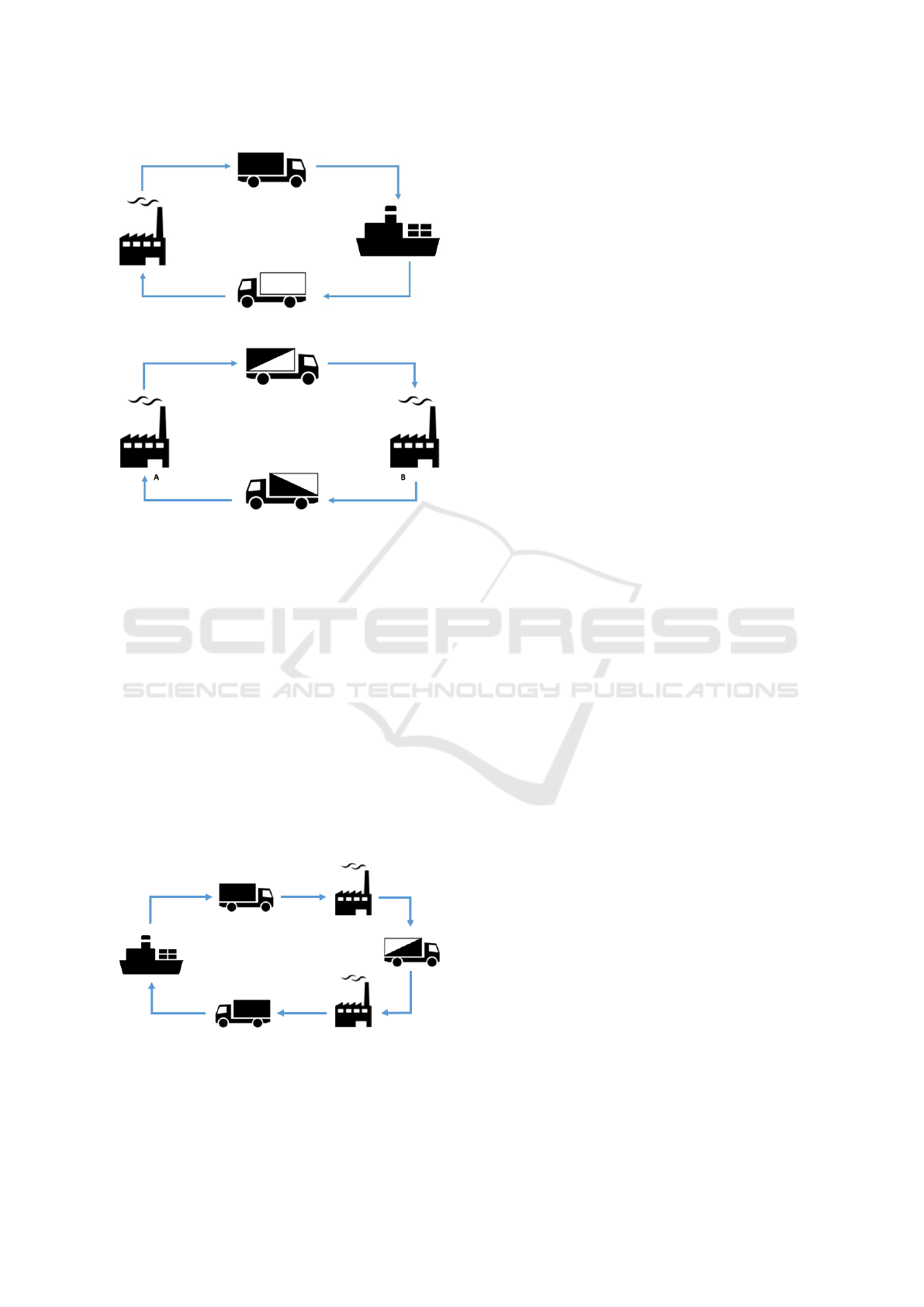
Figure 2: Export scenario.

Figure 3: Inland trips.

trucks and the road network. It may be the case that

a customer that exports goods does not import any

goods, at least not from the same port. But generally

the customer demands goods as well, and the truck

may return loaded if it visits a company that sells the

goods the customer needs. Even more, from the port

to that company the truck may bring goods impor-

ted by the company that are on the port waiting to

be transported. Thus, an export trip may be combi-

ned to an import trip, or an import trip followed by

an inland trip, as shown in Figure 4. A perfect com-

bination would include a sequence of trips in which

the destination of a trip is the origin of the next one.

A good combination allows a repositioning trip bet-

ween the end of a trip and the start of the next one, as

long as those locations are not far away, i.e., when the

repositioning may be done by a small trip.

Figure 4: Combination of export, import and inland trips.

The combination of trips becomes an alternative

to avoid such problem. Import and export trips that

would be performed by different trucks may be per-

formed sequentially by the same truck, thus decrea-

sing the number of empty trucks traveling in the road

system, which contributes to the transportation net-

work as a whole (reduction of truck trafﬁc and road

congestion) besides to the environment (reduction of

emission of polluting gases) (Islam, 2017a). Further-

more, Schulte et al. (Schulte et al., 2015) mention that

such combination contributes also to decrease opera-

tional costs and additional gains to drivers.

The objective of this work is to propose a mat-

hematical model to ﬁnd a good (possible the best)

combination of trips (export, import and inland trips)

to reduce empty trucks travelling through the roads,

which besides the contributions aforementioned, may

reduce the waiting time in ports and congestion in

ports area. The model includes constraints to assure

drivers welfare by enforcing current laws regulation.

This paper is organized as follows: in Section 2

we present related works from the literature; a for-

mal deﬁnition of the problem is presented in Section

3; in the following, in Section 4, the proposed met-

hod is described, which consists of a mixed integer

linear programming, a heuristic for evaluating each

possible combination of trips, and an integer linear

programming for choosing a set of those combinati-

ons; experimental results are presented in Section 5

and conclusions and future works in Section 6.

2 LITERATURE REVIEW

The combination of trips to decrease empty trucks

traveling along the roads have already been addres-

sed in the literature. Gavish and Schweitzer (Gavish

and Schweitzer, 1974) are among the ﬁrst to propose

such approach.

Ozener and Ergun (

Ozener and Ergun,

2008) study a logistic network in which shippers col-

laborate to share a common carrier. Their study has

identiﬁed routes in which a collaborative scheme may

reduce the shared costs among shippers. Audy et al.

(Audy et al., 2011) shows that in their context both

the cost and the delivery time may be reduced using

collaborative transportation.

Caballini et al. (Caballini et al., 2015) studied a

problem similar to the one we study here, with ex-

port, import and inland trips in a port context, where

all trucks may transport two 20 ft containers. They

proposed a Mixed Integer Linear Programming for-

mulation (MILP) to minimize the overall costs of trips

subject to time windows and time limit in the rou-

tes. They study the impact of trips combination on

real data in the port of Genoa, Italy, showing that trip

combination may reduce the costs and the number of

empty tricks traveling to/from the port.

ICEIS 2018 - 20th International Conference on Enterprise Information Systems

320

Schulte et al. (Schulte et al., 2015) developed si-

mulation models for coordinated truck appointments

and used the proposed approach to solve the problem

as a TSP with time windows allowing collaboration.

They used instances based on real data of the port

of Santo Antonio, Chile, and integrated their appro-

ach to a Truck Apointment System (TAS), a tool to

schedule and follow cargo arriving, allowing collabo-

ration among ports and transportation companies. As

a result, ports could reduce port-related polluting gas

emission using the model in real-time.

Islam (Islam, 2017b) also simulated the sharing of

trucks in a port environment. He compared two scena-

rio, the ﬁrst considering sharing/collaboration and the

second without it. Using data of a local port, he sho-

wed that the collaboration between trucks increases

the use of the port capacity as well reduces polluting

gas emission and congestion around the port.

A more recent work of Caballini et al. (Cabal-

lini et al., 2017) proposes a model to reduce costs and

the number of trips that trucks travel empty, take ad-

vantage of the capacity of the trucks. They show the

efﬁcacy of the proposed approach by computational

experiments.

The present work differs from the ones cited above

by including local transport regulation laws and time

windows, thus adapting previous ideas towards the

Brazilian exportation context. Caballini et al. (Ca-

ballini et al., 2015) is the one more similar, but here

we include a heuristic phase, due the complexity of

the resuling model, when all considered characteristis

are included.

3 PROBLEM DEFINITION

We are given as input a set T of trips. For each

trip i ∈ T we have its origin and destination location,

respectively O

and D

, and the distance d

between

those locations, in Km. We also have the distance e

between the destination of a trip i ∈ T and the ori-

gin of a trip l ∈ T \i, also in Km. This distance is

traveled by a truck covering two trips i, l sequentially

when D

6= O

(considered 0 when they coincide) and

is called repositioning trip. The duration of each trip

i is deﬁned by t

= d

/speed, and the duration of re-

positioning trip is e

/speed. In all cases we consider

a constant speed of 80 km/h. This is in fact the max-

imum speed for heavy trucks in Brazilian roads, but

as most of the trips are long distance trips, trucks will

using this speed most of the time, and then may be

used as average speed. Moreover, there is a service

time S that is including in all trips, covering the loa-

ding and unloading service at cities and ports.

Trips are under transport regulation laws that im-

pose 30 min of rest after each 5,5 hours of travel, and

8 hours after each 12 hours. The ﬁrst one imposes a

small rest during a trip, and the second one a long rest

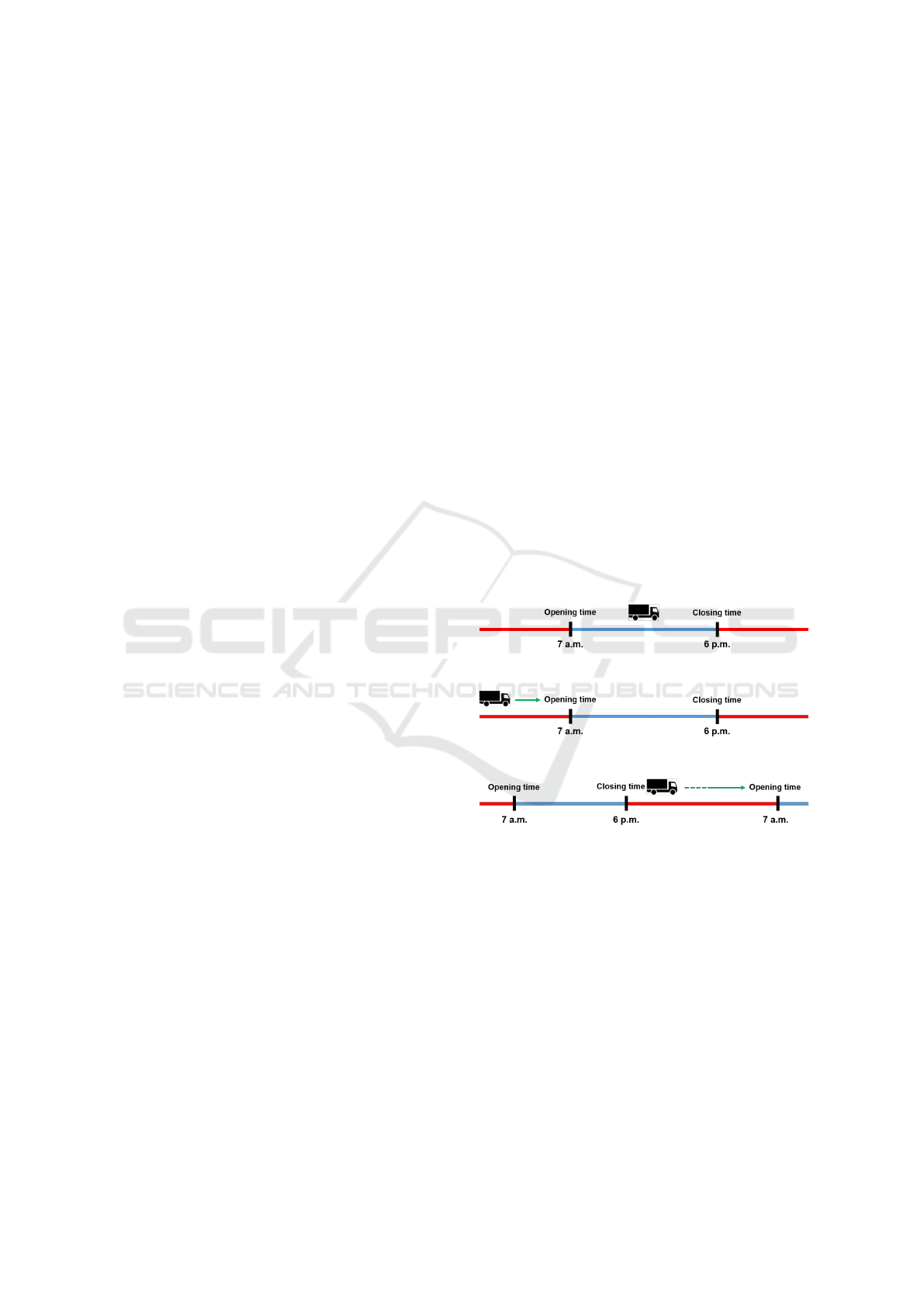
(night/sleep resting, for example). Besides mandatory

resting times, drivers are subject to waiting times due

to opening and closing time of locations (deposit in

cities and ports). For each location there is a time win-

dow, and operations may be done only inside the time

window. This is represented in Figure 5; in this case,

the truck arrived within the time window. For each

trip i we know the time window of the origin location,

], and of the destination location, [P

]. If

the truck arrives before the opening time, it must wait

until the window opens (see Figure 6). If the truck

arrives after the closing time, it must wait until the

next day, for the following time window, as represen-

ted in Figure 7. This may happen also when starting

a trip and in repositioning trips. Those waiting times

are added to the total duration of the combination of

trips. For some trips there is a good combination to

avoid those wasted time, but for some the total du-

ration time may include many hours due to waiting

times. The choice of combinations must be carefully

done to avoid or minimize that.

Figure 5: Trip arriving inside the time window.

Figure 6: Trip arriving before the time window.

Figure 7: Trip arriving after the time window.

We consider combinations of at most 3 trips. A

good example of combination of 3 trips is the one de-

picted in Figure 4 where an import trip is followed

by an inland trip and then an export trip. This case

happens when the destination of the ﬁrst trip does not

have any goods to send to the port. Instead of co-

ming back to the port empty, the driver travels to a

nearby city and carries the truck with goods prepa-

red for exportation. Another case is the combination

of export/inland/inland trips: a rural producer exports

goods and imports agricultural inputs; after unloading

the goods at the port, the driver travels to a nearby city

to load the agricultural inputs to bring to the producer.

A combination of more than 3 trips would include a

Reducing Empty Truck Trips in Long Distance Network by Combining Trips

321

double trip to the port or from the port, which can be

modeled as two combinations.

The objective is then to ﬁnd the best combinations

of trips in order to minimize the total duration time,

considering the duration of all combinations chosen

and trips performed as single trip, if a trip is chosen

not to be combined. The formal deﬁnition of the ob-

jective and the aforementioned constraints is detailed

in the MILP formulations proposed in the following

section.

4 SOLUTION METHOD

Our ﬁrst attempt was to propose a MILP formula-

tion that includes all characteristics of the problem,

as the one proposed by Caballini et al. (Caballini

et al., 2015). The formulation had variables to cont-

rol which trips belongs to each combination and their

sequence in the combination. Moreover there were

a considerable number of variables to control res-

ting/waiting time within trips (following law regula-

tions) and between trips (due to time windows). Ho-

wever, we are working with a more complex problem,

mainly because we have to deal with some very long

distance trips, that may spam more than one day, even

when performed as a single trip. The control of the

starting and ending of each trip becomes more com-

plex due to different restring times that are manda-

tory along the way. Although we could indeed include

all characteristics in a MILP formulation, it turns out

to solve only instances with very small number of

trips, and using a long CPU time. Nevertheless we

can still solve the problem using exact MILP formu-

lation by decomposing the problem: ﬁrstly we do a

pre-processing to determine the best way to combine

each sequence of 2 or 3 trips, and then we search the

best set of combinations that covers all trips at a mi-

nimum cost.

For the ﬁrst phase, we propose a MILP formula-

tion to determine the best duration of a given sequence

of trips. This includes determining the best starting

and ending time of each trip in order to reduce the

total duration time. The proposed formulation is pre-

sented in Section 4.1. Although the formulation can

handle at a reasonable time all the subsets of 2 or 3

trips, it may be impracticable to use it for large in-

stances because of the exponential number of possi-

ble combinations to be solved. We then propose, at

Section 4.2, a constructive heuristic to be used when

needed as an alternative in this phase. After the pre-

processing phase, independently of the method used,

a set-covering based formulation (Section 4.3) is used

to determine the best set to cover all trips.

4.1 Pre-processing Combinations

In order to choose the best combinations for a given

set of trips, we ﬁrst do a pre-processing to deﬁne the

optimal cost (in terms of total duration) for each pos-

sible combination of 2 or 3 trips, i.e., we generate all

sequence of 2 and 3 trips, and for each one of them,

we evaluate its total duration time by deciding the

start and ﬁnish time of each trip, besides the resting

and waiting times. In this section we describe a MILP

formulation for this task, and in the following section

we describe a greedy constructive heuristic.

We propose the following MILP formulation to

deﬁne the minimal cost for the combination of trips

i,l,k ∈ T sequentially.

We use indexes i,il,ilk when describing variables

or data respectively for trip i, trip l (performed after

i) and trip k (performed after i and l). For example,

if q denotes the starting time of a trip, q

and q

ilk

denote the starting time of trips i,l,k in the combina-

tion. Moreover, we use

to indicate a given time in a

day, i.e., remaining hours discounting full days. For

example, if q

ilk

= 83, the starting time of trip k is 83

hours after time 0 of the planning horizon, i.e., 3 days

and 11 hours, then q

ilk

= 11.

We use the following decision variables:

q: starting time of a trip;

: starting hour of a trip;

f : ending time of a trip;

: ending hour of a trip;

: resting time of a daily journey (8h every 12h);

: resting time during a trip (30’ every 5:30h);

: waiting time to start a trip;

: waiting time after ﬁnishing a trip;

: binary, if a trip ends before time window;

: binary, if a trip ends after time window;

: binary, if a trip is ready to start before time

window;

: binary, if a trip is ready to start after time win-

dow;

z: number of full days of a given duration time;

: number of required resting periods;

The constraints below show how f

is deﬁned

from f

(1)-(2), how binaries b

and a

are set when

trip i did not ﬁnish within the operation time [P

]

of the destination of trip i (3)-(6) and how the waiting

time is set in these cases (7): the remaining hours until

the opening time if arrived early, or the hours until the

ICEIS 2018 - 20th International Conference on Enterprise Information Systems

322

opening time of the next day if arrive tardy. Similar

constraints are deﬁned for f

, f

ilk

= f

/24 (1)

= f

− 24bz

c (2)

≤ P

(3)

≥ P

(1 − b

) (4)

(24 − f

≥ (24 − P

) (5)

24 − f

≥ (24 − P

)(1 − a

) (6)

= (P

− f

+ (24 − f

+ P

(7)

∈ {0, 1} (8)

∈ {0, 1} (9)

≥ 0 (10)

The integer value z

= bz

c may be deﬁned for a

continuous value z

by the constraint z

− 1 ≤ z

≤ z

The following expressions deﬁne the total resting

time of different types while performing trip i. Si-

milar expressions are used for trips l and k (variables

ilk

= t

/12 (11)

= t

/5.5 (12)

= 8bm

c (13)

= 0.5bm

c (14)

The complete MILP formulation is then:

min B

ilk

= ( f

ilk

+ w

ilk

− q

) (15)

subject to:

≤ q

≤ P

(16)

= q

+ r

(17)

= f

+ w

+ e

+ r

+ s (18)

= q

+ w

+ r

(19)

ilk

= f

+ w

+ e

+ r

ilk

+ r

ilk

+ s (20)

ilk

= q

ilk

+ w

ilk

+ r

ilk

+ r

ilk

(21)

(22)

(1)-(9) for f

, f

ilk

(11)-(14) for r

ilk

, f

ilk

, f

ilk

≥ 0 (23)

ilk

≥ 0 (24)

Objective function (15) minimizes the cost (total

duration time) of the combination. The starting time

of the ﬁrst trip, i, must be within the operation hour of

the origin location of the trip (16). The ﬁnishing time

of this trip is the starting time plus the time needed to

go from its origin to its destination plus the mandatory

resting times (17). As for the next trip, l, it may start

after ﬁnishing the previous one, plus the repositioning

time from the destination of i to the origin of l plus the

resting times, if any, during this repositioning (18).

Constraints (19)-(21) do the same for other trips.

We run the above formulation for all triplets

i,l,k ∈ T . If the solution is feasible, we have the mini-

mal cost B

ilk

of the combination. Otherwise we have

that trips i.l.k cannot be combined sequentially.

The MILP formulation to deﬁne the minimal cost

for the combination of two trips i,l ∈ T is similar:

min C

= f

+ w

− q

(25)

subject to all constraints except the ones including va-

riables with index ilk.

4.2 Pre-processing Heuristically

Here we propose a greedy constructive heuristic to

quickly deﬁne an upper bound on the cost and total

duration of a sequence of trips i,l,k, considering that

each trip departs and a arrives as early as possible.

For example, the starting time of the ﬁrst trip is the

opening time of its origin point: q

= P

. The en-

ding time f

includes the service time, the distance

to the destination point, mandatory resting time, and

waiting time due to time windows. The starting time

of the following trips include also the repositioning

from the destination point of the previous trip and the

possible incurring resting and waiting time.

It is easy to see that this heuristic gives an up-

per bound on the cost/total duration because the se-

quence thereby constructed is feasible: all constraints

are considered. One may also notice that it may not

be optimal, because starting a trip as early as possible

may force waiting times in the future that may incre-

ase the total duration time. It is, however, very fast.

Therefore we have an exact ILP formulation that,

given a set of trips i,l,k determine the best star-

ting/end time of each trip in order to minimize the

cost (albeit costly in terms of computational time),

and a heuristic that quickly determines a possible

good value. Regardless the method used for this pre-

processing time, or even a mixed of both, we still have

to decide which trips to combine. This task is done by

the set-covering based ILP formulation given in the

next section.

4.3 Set-covering ILP Formulation

After pre-processing all combinations up to 3 trips, let

and T

be the sets of all feasible combinations of

Reducing Empty Truck Trips in Long Distance Network by Combining Trips

323

2 and 3 trips respectively, and let B

ilk

be the total cost

of combining trips i,l,k sequentially, C

the total cost

of combining trips i,l sequentially, and D

the cost of

a single travel i (in our case twice the distance because

it would be a round trip). We then deﬁne the following

compact ILP formulation, using variables v

and y

ilk

as binary decision variables equals to 1 if trips i,l and

i,l,k respectively are to be combined and 0 otherwise,

and x

a binary decision variable equals to 1 if the trip

i is to be performed as a single trip (i.e., not part of

any combination) and 0 otherwise.

min Z =

∑

ilk∈T

ilk

∑

il∈T

∑

i∈T

(26)

subject to:

∑

ilk∈T

i= j∨l= j∨k= j

ilk

∑

il∈T

i= j∨l= j

+ x

= 1 ∀ j ∈ T (27)

ilk

∈ {0, 1} (28)

Objective function (26) minimizes the overall

cost. Constraints (27) state that each trip may be at

most in one chosen combination or performed as a

single trip. The last constraints state that all variables

are binary.

5 EXPERIMENTAL RESULTS

The MILP formulations were implemented in C/C++

using the Concert Technology Library, and solved by

CPLEX 12.5 academic license. The heuristic was im-

plemented in C/C++. The experiments were run on an

IntelR Core TM i7-4790K CPU @ 4.00GHz x 8 with

32GB RAM, running Ubuntu 14.04 LTS 64 bits.

5.1 Instances

We generate a set of instances based on real data

from the Brazilian transportation network. Data were

collected from Fretebras

, a website containing thou-

sands of freightage offers, ﬁlled by drivers and com-

panies in real-time, covering all Brazilian states and

some nearby countries. One may freely consults in-

formation such as origin and destination of freightage,

distance between those sites, vehicle type, freight

type, and others.

We selected 10 cities, including Santos - SP, Cu-

bat

ao - SP, Manhuac¸u - MG, Passos - MG, Arcos -

MG, Rondon

opolis - MT, Sorriso - MT, Dourados -

MS and Itumbiara - GO, which are among the main

http://www.fretebras.com.br

origin or destination points for export of grains (cof-

fee and soy), and import of agricultural inputs (ferti-

lizers and agricultural plaster), thus generating most

of the import and export trips on the roads network of

the southeast region of Brazil. Santos is a port city

that receive plenty of trucks everyday, both for import

and export freights. We created seven instances, ran-

ging from 7 to 124 trips, using data from selected trips

of the Fretebras website.

The distances of the trips range from 20 to 2246

km, while the estimated duration ranges from 15 min

to almost 30 hours (including the repositioning trips,

which can be very short). Table 1 shows a summary

of the data for each instance, considering the import,

export and inland trips.

Table 1: Summary of the instances.

ID # Trips

Duration (h)

min max avg

1 15

3.7 26.7

14.0

2 31 15.8

3 47 14.5

4 62 13.1

5 76 15.0

6 94 13.5

7 124 13.9

We consider the same operation time for all cities:

7 am as the opening time and 6 pm as the closing time.

5.2 Results

The instances were solved by the two approaches pro-

posed: pre-processing the combinations by the exact

ILP model or the constructive heuristic and then se-

lect a subset of combinations by the set-covering mo-

del. The results are presented in Table 2, for 4 types

of tests: trips allowed to combine in sequence of 2

and/or 3 trips; trips allowed to combine only in se-

quence of 3 trips; only in sequence of 2 trips; and no

combination allowed (last rows, combined type = 1).

Notice that for this last type, none of the formulations

or approaches are used, one truck is used for each trip,

and the total cost may be evaluated at practically zero

time.

For each type of test, we report the objective

function value (accumulated duration time of all

trips), the number of trucks used, and the total time for

each approach for pre-processing: MILP of Section

4.1 and Heuristic (Heur) of Section 4.2. We do not

report gaps of the formulations because all formulati-

ons were solved until a proved optimal is found. For

the case of no combination (type 1), each trip is con-

sidered as a round trip, then the duration of a trip is

twice the travel time and mandatory resting and wai-

ting times.

ICEIS 2018 - 20th International Conference on Enterprise Information Systems

324

From the results we can see that for all instan-

ces, the proposed approaches could combine the trips,

decreasing the overall duration time and the number

of trucks, compared to the case of no combinations.

This can be seen on the table, and on Figures 8 and 9,

which show respectively the objective value and num-

ber of trucks for all instances and combination types.

In Figure 8, the objective values were scaled to the

cost of the 1-type, which was always the highest. In

order to have a clearer visualization of the results for

the number of trucks, Figure 10 shows the results only

for types that allow combinations.

The combination type that reached the minimum

objective value was, as expected, the 2&3 combina-

tion type, when pre-processing is done exactly. This

can be seen on the table and on the graphic of Figure

8. However, the combination that minimizes the most

the number of trucks was the 3-combination type,

which can be seen on the table and on the graphic of

Figure 10.

We may conclude that, using only combinations

of 3 trips, we may minimize the number of trucks, but

this may not be the best option in terms of total time.

In some cases a third trip may force a long waiting

time, and the best option is to combine only two trips.

Therefore, we have to allow combinations of 2 and of

3 trips, if we want to reduce the overall time.

In general, results obtained by pre-processing

using heuristics have higher objective values, regard-

less the combination type (see Figure 8). This hap-

pens because not all trips are combined. In the other

hand, pre-processing the combinations by the exact

ILP formulation yields lower costs for each combina-

tion, and the result is that in the second phase almost

all trips are combined, reducing the overall costs.

The exact pre-processing, however, is computati-

onal costly. For the larger instances, the exponential

number of combinations and the high cost to solve all

of them, lead the algorithm to run for more than one

day, reaching almost one week for the largest instance

allowing 3 or 2&3 combinations. The running time of

the heuristic was at most 2 minutes.

The approach here proposed reached all the ex-

pected objectives, while satisfying the imposed con-

straints:

• Minimization of costs

The combination of trips allows a given driver to

perform two or three trips. Doing this, we avoid to

use a new driver to cover some trips, reducing the

operational costs. Another reason is the smaller

distances traveled for repositioning trips, which

reduces empty truck trips.

• Minimization of empty truck trips and maximiza-

tion of the use of trucks capacity

When choosing the best combined route, the mo-

del prefers low cost combinations. A low cost

combination has generally a small distance for re-

positioning or no repositioning at all. As those tra-

vel times are considered in the objective function,

a preference is given for smaller distance for repo-

sitioning (which is also empty truck trips), using

the capacity of trucks as long as possible.

• Minimization of polluting gas emission

This is a direct consequence of the combination

of trips. As well as the reduction of the number

of drivers, lesser vehicles on the road reduces the

emission of polluting gases. Another cause is the

reduction on the number and distance travelled on

repositioning trips.

• Minimization of waiting on port area

The proposed approach takes in account the arri-

ving and departure time on ports and cities. When

a trip arrives outside the time window, the waiting

time is added to the objective function. Therefore,

the waiting time is reduced in order to minimize

the overall time. Moreover, the formulation deci-

des also the best departure time of the ﬁrst trip,

aiming to minimize the required waiting time.

• Solutions conforme to Brazilian transport regula-

tion laws

The formulation include regulations of the Brazi-

lian transport law 13103/2015, adding the manda-

tory resting periods. This includes daily rests, of

30 minutes for each 5:30h of driving, and long rest

of 8h after 12h driving.

Figure 8: Objective value.

6 CONCLUSIONS

This paper proposes a mathematical programming

formulation to meet the needs of a transportation net-

work including export, import and inland trips. The

main objective is to reduce empty truck trips, i.e., the

number and distance traveled by empty trucks. This

Reducing Empty Truck Trips in Long Distance Network by Combining Trips

325

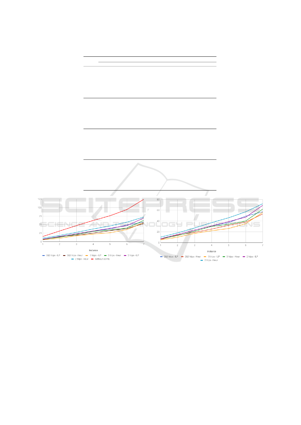
Table 2: Experimental results for all instances, approaches and combinations type.

Comb. Instance Total duration CPU time (s) #Trucks

type ID Size ILP Heur ILP Heur ILP Heur

1 15 318.5 339.2 28 <1 7 6

2 31 720.1 807.1 394 <1 15 14

3 47 1033.7 1082.6 2789 4 23 19

2&3 4 62 1241.6 1388.3 10792 12 31 25

5 76 1740.5 1841.0 44535 20 37 32

6 94 1832.3 1998.2 110329 49 44 38

7 124 2122.3 2783.5 591482 170 57 53

1 15 323.2 341.7 33 <1 7 7

2 31 790.0 829.9 402 <1 10 13

3 47 1058.0 1110.2 2840 2 17 21

3 4 62 1268.2 1379.7 10829 8 22 30

5 76 1767.8 1865.5 33358 13 26 34

6 94 1928.4 2033.1 112263 35 32 40

7 124 2642.4 2906.2 544535 104 42 62

1 15 320.7 372.5 <1 <1 7 10

2 31 774.3 813.3 4 <1 15 18

3 47 1035.9 1113.8 19 2 23 27

2 4 62 1241.6 1379.4 56 5 31 37

5 76 1742.7 1881.9 134 8 39 1/46

6 94 1876.6 2047.0 356 21 47 57

7 124 2584.6 2862.4 1329 76 62 72

1 15 594.3 - - 15

2 31 486.7 - - 31

3 47 2975.6 - - 47

1 4 62 2290.6 - - 62

5 76 3320.7 - - 76

6 94 3538.8 - - 94

7 124 4859.6 - - 124

Figure 9: Number of trucks for all combination types, in-

cluding no combinations.

task was accomplished by minimizing the total dura-

tion of trips, which forces the combination of 2 or 3

trips in order to avoid needless trips. The combina-

tion was done respecting regulation laws imposed to

drivers traveling long distances and also the operation

times of ports. Using real-based data of Brazilian sce-

nery, we show that the number of empty trucks was

reduced, which directly contributes to reduce the con-

gestion on port areas and polluting gases emission.

For a small number of trips, the MILP formulation

showed to be a useful tool for route planning. But as

the number of trips increase, the computational time

becomes impracticable. In such case, a fast heuristic

may ﬁnd a reasonable solution, not far from the opti-

mal, in short computational time.

Figure 10: Number of trucks for all combination types.

As future works we plan to improve the model in

order to reduce the computational time, and use ot-

her strategies to reach the optimal solution, for exam-

ple dynamic programming. Other work would be to

improve the quality of the heuristic, maintaining the

short computational time. This would allow the set-

cover formulation to be used in almost real-time for

replanning the combination in case of eventualities.

A further step would be to assign the combinations or

sequence of combinations of trips to a set of drivers.

In this last case, we may have to use metaheuristics,

as the problem may become more complex and a sim-

ple greedy heuristic, despite the good results achieved

in this paper, may not give a good result in this more

complex scenery.

ICEIS 2018 - 20th International Conference on Enterprise Information Systems

326

ACKNOWLEDGEMENTS

The authors thank Coordenac¸

ao de Aperfeic¸oamento

de Pessoal de N

ıvel Superior (CAPES) and Fundac¸

de Amparo

a Pesquisa do Estado de Minas Gerais

(FAPEMIG) for the ﬁnancial support of this project.

The ﬁrst author thanks Gilson F. Ataliba for his con-

tribution in the ﬁrst ILP formulation.

REFERENCES

Audy, J.-F., DAmours, S., and Rousseau, L.-M. (2011).

Cost allocation in the establishment of a collabora-

tive transportation agreementan application in the fur-

niture industry. Journal of the Operational Research

Society, 62(6):960–970.

Caballini, C., Paolucci, M., Sacone, S., and Ursavas, E.

(2017). Towards the physical internet paradigm: A

model for transportation planning in complex road

networks with empty return optimization. In Interna-

tional Conference on Computational Logistics, pages

452–467. Springer.

Caballini, C., Rebecchi, I., and Sacone, S. (2015). Combi-

ning multiple trips in a port environment for empty

movements minimization. Transportation Research

Procedia, 10:694–703.

Caixeta Filho, J. V. (2010). Log

ıstica para a agricultura bra-

sileira. Revista Brasileira de Com

ercio Exterior.

Gavish, B. and Schweitzer, P. (1974). An algorithm for

combining truck trips. Transportation Science, 8.

Islam, S. (2017a). Empty truck trips problem at container

terminals: A review of causes, beneﬁts, constraints

and solution approaches. Business Process Manage-

ment Journal, 23.

Islam, S. (2017b). Simulation of truck arrival process at

a seaport: evaluating truck-sharing beneﬁts for empty

trips reduction. International Journal of Logistics Re-

search and Applications, pages 1–19.

Ozener, O.

O. and Ergun,

O. (2008). Allocating costs in

a collaborative transportation procurement network.

Transportation Science, 42(2):146–165.

Schulte, F., Gonz

alez, R. G., and Voß, S. (2015). Redu-

cing port-related truck emissions: coordinated truck

appointments to reduce empty truck trips. In Interna-

tional Conference on Computational Logistics, pages

495–509, The Netherlands. Springer.

Reducing Empty Truck Trips in Long Distance Network by Combining Trips

327