
Travel Time Modeling using Spatiotemporal Speed Variation and a
Mixture of Linear Regressions
Mohammed Elhenawy
1
, Abdallah A. Hassan
2
and Hesham A. Rakha
1,3
1
Virginia Tech Transportation Institute, 3500 Transportation Research Plaza, Blacksburg, VA 24061. U.S.A.
2
Bradley Department of Electrical and Computer Engineering, Electrical & Computer Engineering,
MC 0111, 1185 Perry St., Blacksburg, VA 24061, U.S.A.
3
Charles E. Via, Jr. Department of Civil and Environmental Engineering, Blacksburg, VA 24061, U.S.A.
Keywords: Travel Time Modelling, Travel Time Reliability, Spatiotemporal Speed Matrix, Mixture of Linear
Regressions.
Abstract: Real-time, accurate travel time prediction algorithms are needed for individual travelers, business sectors,
and government agencies. They help commuters make better travel decisions, avert traffic congestion, help
the environment by reducing carbon emissions, and improve traffic efficiency. Travel time prediction has
begun to attract more attention with the rapid development of intelligent transportation systems (ITSs), and
is considered one of the more important elements required for successful ITS subsystems deployment.
However, the stochastic nature of travel time makes accurate prediction a difficult task. This paper proposes
travel time modeling using a mixture of linear regressions. The proposed model consists of two normal
components. The first component models the congested regime while the other models the free-flow regime.
The means of the two components are modeled by two linear regression equations. The predictors used in
the linear regression equation are selected out of the spatiotemporal speed matrix using a random forest
machine-learning algorithm. The proposed model is tested using archived data from a 74.4-mile freeway
stretch of I-66 eastbound connecting I-81 and Washington, D.C. The experimental results show the ability
of the model to capture the stochastic nature of travel time and to predict travel time accurately.
1 INTRODUCTION
Minimizing drivers’ travel times from their origins
to their destinations is a major Intelligent
Transportation Systems (ITSs) objective. However,
it is also extremely challenging due to the dynamic
nature of traffic flow, which is, in most cases, highly
unpredictable. One straightforward strategy involves
directing vehicles or guiding drivers to follow routes
that avoid congested paths. A critical step for this
route planning or guidance to be effective is the
ability to accurately predict travel times of different
alternative routes from source to destination.
In addition, travel time represents an important
performance measure for traffic system evaluation.
It is easily understood by drivers and operators of
traffic management systems, and can be viewed as a
simple summary of a traffic system’s complex
behavior. In order for an ITS to accurately predict
the travel time, it must have the following
capabilities, each of which comes with associated
difficulties:
1. Sensing and acquiring the current state of
the transportation network of interest where
a number of data values need to be detected
and collected, including traffic conditions
and parameters at different parts of the
network, whether some roads are currently
congested, current weather conditions, time
of day, whether there is an incident on any
road in the network, etc. Gathering such
data on every road and intersection with the
quality that allows accurate forecasting of
travel time between two points in the
network may be fairly expensive.
2. Storing a long history of traffic parameters
for the transportation network of interest to
support future prediction of travel times.
This historical dataset may be large and
difficult to use and manage.
Elhenawy, M., Hassan, A. and A. Rakha, H.
Travel Time Modeling using Spatiotemporal Speed Variation and a Mixture of Linear Regressions.
DOI: 10.5220/0006690601130120
In Proceedings of the 4th International Conference on Vehicle Technology and Intelligent Transport Systems (VEHITS 2018), pages 113-120
ISBN: 978-989-758-293-6
Copyright
c
2019 by SCITEPRESS – Science and Technology Publications, Lda. All rights reserved
113

3. Feeding the current state of the network
along with its traffic history to some type of
model that predicts travel time if a trip will
start from some point and end in another in
the network at some specific time.
Designing such a model is challenging, as
is finding a set of current or historical
parameters with real prediction power. The
most useful model may be road dependent,
and even for a single road, it has been
shown that different models may describe
the traffic behavior more accurately at
different traffic conditions. For instance,
one model may be more useful when the
road is congested, while another model may
be more accurate when vehicles are flowing
freely, etc.
In short, accurate traffic time prediction is
challenging due to the high cost of sensing and
collecting enough useful current and historical
traffic data. Even when such data is available, it is
still difficult to determine which type of model best
describes the traffic behavior, and which traffic
parameters should be fed to the model for the best
predictions. Moreover, the best course of action may
be to use two or more models and switch between
them depending on current traffic conditions. This
option adds a new challenge, as it is necessary to
decide which model from the set of models will be
used for some specific input data, or whether
different models will be used for prediction with
some weight applied to each output prediction to
reach a final travel time prediction.
In this paper, a new method for travel time
prediction is proposed. This method uses a mixture
of linear regressions motivated by the fact that travel
time distribution is not unimodal, since two modes
or regimes of traffic can exist—one at congestion
state, and the other at free-flow state. The proposed
model was built and tested using probe data
provided by INRIX and supplemented with
traditional road sensor data as well as mobile
devices and other sources. The dataset was collected
from a freeway stretch of I-66 eastbound connecting
I-81 and Washington, D.C. The traffic on this stretch
is often extremely heavy, which makes travel time
prediction more challenging, but also makes the data
more valuable and helps create a more realistic
model.
2 RELATED WORK
Various methods and algorithms have been proposed
in the literature for travel time prediction. These
methods can roughly be classified into two main
categories: statistical-based data-driven methods and
simulation-based methods. This section focuses on
the statistical-based methods since the proposed
solution in this paper falls under this class of
methods, and because more research in the literature
uses statistical methods.
Several researchers fit different regression
models to predict travel time. A typical approach is
to fit a multiple linear regression (MLR) model
using explanatory variables representing
instantaneous traffic state and historical traffic data,
as, for example, (Rice and van Zwet, 2004, Zhang
and Rice, 2003) . The model proposed in (1) was
even able to use a single linear regression (SLR) to
successfully provide acceptable travel time
predictions. Some researchers developed hybrid
methods where a regression model was used in
conjunction with other advanced statistical methods.
For example, (Kwon et al., 2000) used regression
with statistical tree methods. Another approach
(Chakroborty and Kikuchi, 2004) proposed an SLR
model using bus travel time to predict automobile
travel time.
Regression models are generally powerful in
predicting travel time for short-term prediction,
whereas long-term predictions are less accurate.
Regression models are also reported to be more
suitable for use in free-flow rather than congested
traffic, and fail to accurately predict when incidents
have occurred (Guin et al., 2013).
The idea of using a mixture models for different
traffic regimes has also previously been explored
(Guo et al., 2012). The model developed in this
paper attempts to overcome the drawbacks of
previous work that used mixture models of two or
three components to model travel time reliability,
which suffer from the following limitations:
1. The mean of each component is not
modeled as a function of the available
predictors.
2. The proportion variable is fixed at each
time slot, which limits the model’s
flexibility.
3. Information provided given the time slot of
the day is the probability of each
component (fixed) and the 90th percentile.
Another class of statistical-based methods in
literature uses time series models for travel time
prediction, using, for example, auto-regressive
prediction models (Oda, 1990, Iwasaki and Shirao,
1996, D'Angelo et al., 1999), multivariate time series
models (Al-Deek et al., 1998), and the auto-
VEHITS 2018 - 4th International Conference on Vehicle Technology and Intelligent Transport Systems
114

regressive integrated moving average (ARIMA)
technique (Williams and Hoel, 2003). Similar to
regression models, time series models are more
suitable for free-flow traffic than for congested
traffic, may fail with unusual incidents, and are more
accurate for short-term predictions (Guin et al.,
2013).
Another common technique used for travel time
prediction is the use of artificial neural networks. A
feed-forward neural network is used in (A Cherrett
et al., 1996) to predict journey time. Later, more
advanced neural network techniques were used to
model and predict travel time (Rilett and Park, 2001,
Matsui, 1998, You and Kim, 2000, Guiyan and
Ruoqi, 2003, Guiyan and Ruoqi, 2001, Wei et al.,
2003, . Kisgyorgy and Rilett, 2002). Accurate
predictions were achieved for most proposed
models; for example, in (Kisgyörgy and Rilett,
2002) the prediction error was only 4%.
3 METHODS
In this section, we present a brief introduction of the
powerful modeling techniques used in this paper.
The random forest machine-learning algorithm (RF)
is used to select a subset of important predictors for
travel time modeling. Expectation-maximization
(EM) is used to fit the mixture of linear regression
models to the historical data. The techniques used
are among a number of machine learning and
statistical learning techniques representative of the
wide variety of algorithms that can be used by
transportation practitioners.
3.1 Variables (Predictors) Selection
The I-66 stretch of the freeway section used for this
research consists of 64 segments. The dataset
comprises the spatiotemporal speed matrices for
every day in 2013. The default approach for
modeling and predicting travel time was to take all
the speeds within a window starting right before the
departure time
and covering L past time slots
back to time
. Setting L=30 minutes for
example, the number of predictors will be 64*6 at 5
minutes time aggregation. In order to reduce the
dimensions of the predictors’ vector, RF is used to
select the most important predictors for the travel
time model. Steps to select the most important
predictors are as follows (Breiman, 2001):
1. For each month, build an RF consisting of
100 trees and find the out-of-bag samples
that are not used in the training for each
tree.
2. Find the mean square error
of
the RF using the out-of-bag samples.
3. Randomly permute the value for each
predictor
among the out-of-bag samples
and calculate the mean square error
of the RF.
4. Finally, rank the predictors in descending
order based on the
and choose the top m ranked
predictors.
The higher the predictor’s rank in step 4, the
more important that predictor. The ranking result
shows that, most of the important predictors are
speeds of recent segments (
). In addition to
speed predictors chosen by RF, the historical
average travel time at
given the day of the week is
added as a predictor.
3.2 Mixture of Linear Regressions
A mixture of linear regressions was studied carefully
(De Veaux, 1989, Faria and Soromenho, 2009). It
can be used to model travel time under different
traffic regimes. The mixture of linear regression can
be written as:
(1)
where
is the response corresponding to a vector
of predictors;
,
is the vector of regression
coefficients for the
component and
is mixing
probability of the
component.
The model parameters
={
can
be estimated by maximizing the log-likelihood of
equation (1) given a set of response predictor pairs
using an EM
algorithm. The EM algorithm iteratively finds the
maximum likelihood estimates by alternating the E-
step and M-step. Let
be the parameters’
estimates after the
iteration. In the E-step, the
posterior probability of the
observation from
component is computed using equation (2).
(2)
Travel Time Modeling using Spatiotemporal Speed Variation and a Mixture of Linear Regressions
115
where
is the probability density
function of the
component.
In the M-step, the new parameters' estimates
that maximize the log-likelihood function in
equation (1) are calculated using equations (3-5)
(3)
(4)
where X is the predictors’ matrix with rows
and columns, Y is the corresponding
response vector, and W is a diagonal matrix
which has
on its diagonal.
(5)
The E-step and M-step are alternated repeatedly
until the change in the incomplete log-likelihood is
arbitrarily small as shown in equation (6).
(6)
where is a small number.
4 DATA DESCRIPTION
The freeway stretch of I-66 eastbound connecting I-
81 and Washington, D.C. was selected as the test
site for this study. High traffic volumes are usually
observed during morning and afternoon peak hours
on I-66 heading towards Washington, D.C., making
it an excellent environment to test travel time
models.
The traffic data was provided by INRIX, which
mainly collects probe data by GPS-equipped
vehicles, supplemented with traditional road sensor
data, along with mobile devices and other sources
(INRIX, 2012). The probe data covers 64 freeway
segments with a total length of 74.4 miles. The
average segment length is 1.16 miles, and the length
of each segment is unevenly divided in the raw data
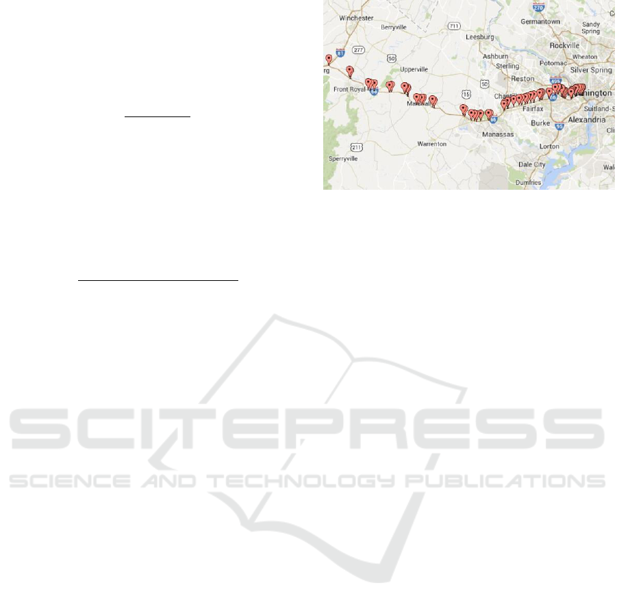
from 0.1 to 8.22 miles. Figure 1 shows the study site
and deployment of roadway segments. The raw data
provides average speed for each roadway segment
and was collected at 1-minute intervals.
Figure 1: The study site on I-66 eastbound (source:
Google Maps).
We sorted the raw data was the roadway
direction according to each TMC station’s
geographic information (e.g., towards eastbound of
I-66). Data was examined to check any overlapping
or inconsistent stations along the route. Afterward,
speed data was aggregated by time intervals (5
minutes in this study) to reduce noise and smooth
measurement errors. This way, the raw data was
aggregated to the form of the daily data matrix along
spatial and temporal intervals. Data was missing in
the developed data matrix, so data input methods
were conducted to estimate the missing data using
values of neighboring cells. Finally, the daily
spatiotemporal traffic state matrix was generated to
model travel time.
5 EXPERIMENTAL WORK
The experimental work is divided into three parts.
The first part is travel time modeling using a mixture
of two linear regressions with fixed proportions
and comparing the proposed model with the
linear regression model. The second part is travel
time modeling using a mixture of two linear
regressions with a variable proportions function of
the same predictors used in the linear regression
equations. The last part explains how the proposed
model can be used to convey travel time reliability
to users.
5.1 Modeling Travel Time using a
Mixture of Linear Regressions with
Fixed Proportions
The purpose of this section is to experimentally
prove that a model using a mixture of two linear
regressions is better than the one component linear
VEHITS 2018 - 4th International Conference on Vehicle Technology and Intelligent Transport Systems
116

regression model. To show that, the proposed model
is fitted to four months of the data then compared to
the linear regression model. Three measures are used
to compare the two models. The Mean Absolute
Percentage Error (MAPE) and the Mean Absolute
Error (MAE) are used to quantify the errors of both
models with respect to the ground truth. MAPE is
the average absolute percentage change between the
predicted
and the true values
. MAE is the
absolute difference between the predicted and the
true values.
(7)
(8)
Here, J is the total number of days in the testing
dataset; I is the total number of time intervals in a
single day; and y and denote the ground truth and
the predicted value, respectively, of the travel time
for the time interval on the day. The lower the value
of these error measures, the better the model.
The other measure used for comparison is the
histogram intersection. It measures how much the
histogram of the predicted travel time, using a
certain model, is similar to the histogram of ground
truth travel time. The higher the value of the
histogram intersection, the better the model,
(9)
where and are the histograms of
ground truth travel time and the predicted travel
time, respectively. Table 1 shows values for the
MAE, MAPE and the histogram intersection for
models using a different number of top ranked
predictors. As shown in Table 1, for all models that
are built using a different number of predictors, the
models built using the proposed mixture of
regressions are better than the linear regression
models with smaller MAE, MAPE and greater
histogram intersection.
5.2 Travel Time Prediction
Modeling travel time allows for travel time
prediction, and conveying this information to
travellers helps them make better decisions. If we
are interested in providing travel time information,
we usually convey the expected travel time as one
value and sometimes also we provide upper and
lower travel time bounds.
Table 1: Comparison between One and Two Components
Models.
MAE
MAPE
Similarity
p
m=1
m=
2
m=1
m=2
m=1
m=2
6
11
16
21
26
31
36
41
46
51
56
61
66
71
76
81
86
91
96
6.57
6.39
6.36
6.32
6.31
6.32
6.30
6.30
6.29
6.23
6.24
6.18
6.18
6.20
6.19
6.20
6.18
6.19
6.19
5.22
5.10
5.05
5.04
5.06
5.09
5.08
5.13
5.12
5.13
5.12
5.16
5.16
5.15
5.15
5.16
5.19
5.21
5.22
7.19
6.99
6.96
6.89
6.90
6.90
6.88
6.88
6.87
6.80
6.82
6.77
6.76
6.79
6.78
6.79
6.78
6.79
6.79
5.69
5.63
5.57
5.56
5.59
5.64
5.62
5.69
5.68
5.70
5.69
5.74
5.74
5.73
5.73
5.74
5.78
5.80
5.80
189
192
196
200
199
198
199
200
200
208
207
215
215
216
215
215
215
214
214
217
223
224
225
227
228
228
231
232
232
232
233
234
234
233
233
233
234
234
Conveying travel time as an interval makes more
sense because it reflects the travel time uncertainty
In this work, for a given unseen new vector of
predictors, the mean of each component is
determined and then travel time is predicted as a
weighted average of the travel time means. The
weights used are the
. The travel time interval for
the unseen predictors' vector is calculated as the
weighted average of the 95% confidence interval for
each component. To evaluate the proposed model in
travel time prediction, the two regression mixture
models are tested using four unseen months. MAPE
and MAE are used to measure expected travel time
accuracy. To evaluate the travel time interval, a
hitting rate measure is defined as the ratio of the
number of ground truth travel times within the
calculated interval to the total number of ground
truth travel times. Table 2 shows the MAPE, MAE,
hitting rate, and travel time width at different
number of predictors. As shown in the table, the
models built using 16 or more predictors have
almost the same accuracy. The parameters' estimates
for the model using a predictor vector of 16
dimensions are shown in Table 3. Figure 2 gives a
better idea of how good the predicted travel times
and intervals are.
Travel Time Modeling using Spatiotemporal Speed Variation and a Mixture of Linear Regressions
117
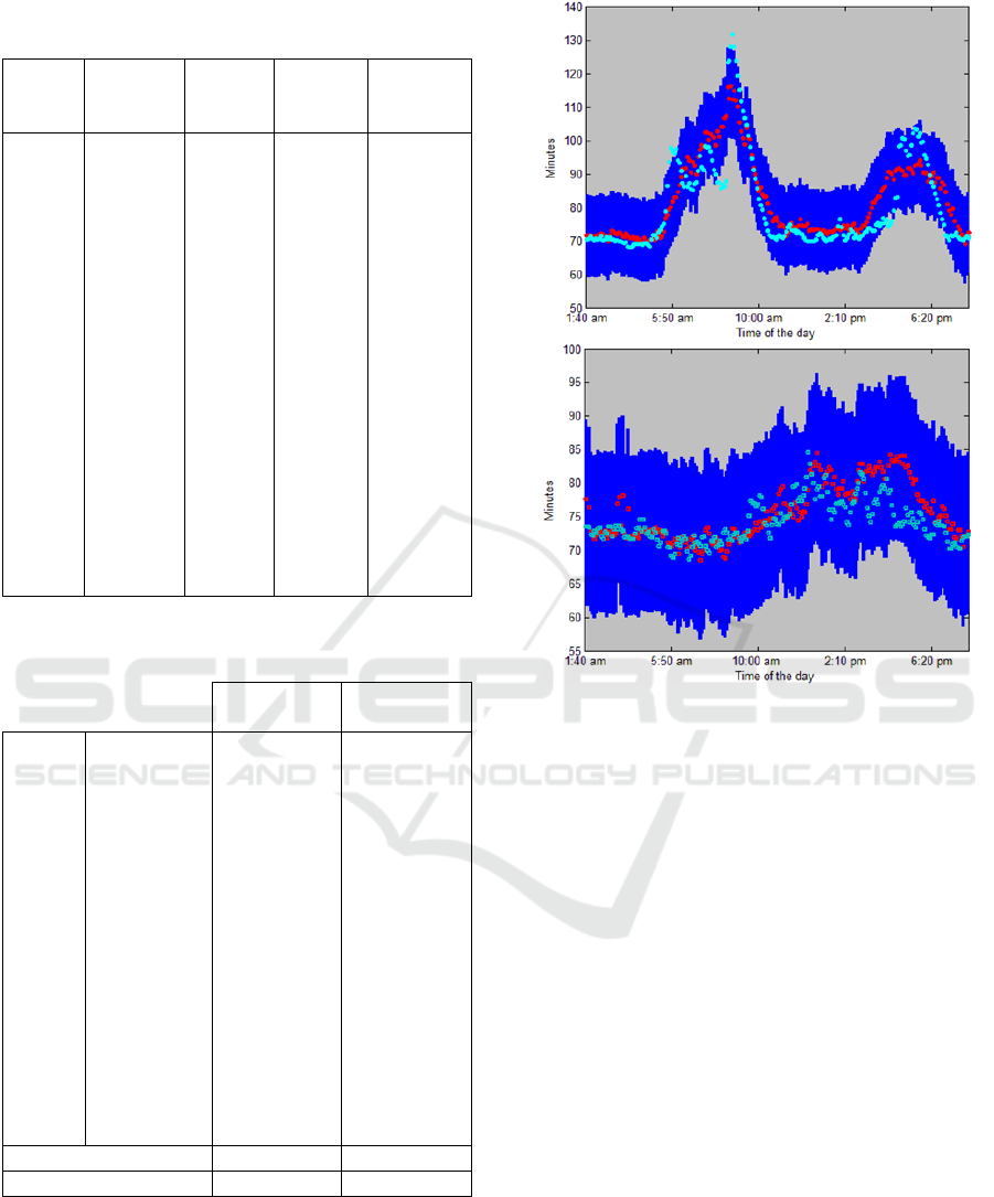
Table 2: Travel Time Accuracy in Terms of MAPE and
MAE, Travel Time Interval's Width and Hitting Rate.
p
MAPE
MAE
% Hitting
rate
Interval
width in
minutes
6
11
16
21
26
31
36
41
46
51
56
61
66
71
76
81
86
91
96
7.97
7.74
7.70
7.70
7.69
7.68
7.67
7.67
7.68
7.68
7.70
7.69
7.69
7.69
7.70
7.71
7.74
7.73
7.73
7.64
7.43
7.39
7.37
7.36
7.35
7.34
7.34
7.34
7.33
7.34
7.32
7.32
7.32
7.32
7.33
7.34
7.33
7.33
81.9
81.1
81.0
80.9
80.8
80.6
80.6
80.4
80.5
80.4
80.5
80.4
80.4
80.4
80.3
80.4
80.2
80.1
80.1
26.4
24.7
24.5
24.4
24.3
24.1
24.1
23.9
23.8
23.8
23.8
23.7
23.7
23.6
23.6
23.5
23.5
23.4
23.4
Table 3: Parameters' Estimates for Mixture of Two
Regressions*.
1st
component
2nd
component
79.4354
-0.0153
-0.0903
-0.0668
-0.0912
0.0187
-0.2107
-0.0652
-0.0245
-0.0106
-0.0745
-0.0174
-0.0203
-0.0742
0.0075
-0.1269
0.6767
96.5943
-0.0148
-0.0250
0.0061
-0.0519
-0.0449
-0.1107
-0.0603
-0.0136
-0.0224
-0.0150
-0.0331
-0.0252
-0.0239
-0.0078
-0.0558
0.0834
11.8066
1.7746
0.4466
0.5534
*(In this table x_(seg#,time) is the speed at certain segment and
time)
Figure 2: Travel time ground truth (red), predicted travel
time (cyan), and travel time interval (blue).
5.3 Travel Time Reliability
Travel time reliability is another piece of
information that can be conveyed to drivers using
the travel time model. Using the proposed model, a
traveler can be informed of probabilities for
congestion and free-flow. Moreover, the expected
and 90th percentile travel times for each regime can
be provided. In order to get good estimates for the
above quantities, the proportions should be functions
of the predictors. Revisiting the EM algorithm, it
estimates the posterior probabilities
and model
parameters, and returns only at convergence
without using
. As shown in equation (4), the
returned
is the average of the posterior
probabilities
. In the two components model, if
is modeled using logistic regression at the
convergence of the EM, this means that
becomes
a function of the predictors as well as the
components' means. Values of
are used, which
result from fitting the model shown in Table 3 to
build a logistic regression. This logistic regression
models the probability of the predictor vector being
VEHITS 2018 - 4th International Conference on Vehicle Technology and Intelligent Transport Systems
118
drawn from component number two. Then, using
simple algebraic manipulation, equation (10) is
derived for
. The new model is the same model in
Table 3 but with variable
and
.
(10)
This model is tested by calculating the mean,
90th percentile, and probabilities of congestion and
free-flow for each predictor vector in each day of
May 2013. Then a day is divided into four time
intervals and the mean of the above quantities is
calculated within each time interval given the day.
The results shown in Table 4 are consistent with the
travel time pattern observed in Table 3, where the
probability of the congestion component increases at
the congestion time of the day. Also, the model
shows that the probability values of morning
congestion during weekends are lower than on
weekdays.
6 CONCLUSIONS
In this paper, we demonstrated the effectiveness of a
travel time model based on a two component
mixture of linear regressions. The proposed model
captures the stochastic nature of travel time, and
assigns one component for the free-flow regime and
the other component for the congested regime. The
means of the components are a function of the input
predictors, which are chosen using a random forest
algorithm. The proposed model can be used to
predict the travel time and the upper and lower
bounds for the travel time as well. Moreover, the
proposed model can be used to provide travel time
reliability information at any time on any day. The
experimental results show the proposed algorithm’s
performance to be promising. The current model
does not consider weather conditions, incidents, or
work zones; however, this model can easily integrate
these factors if a dataset including them is available.
Table 4: Testing the Model for Travel Time Reliability Using May 2013 Data.
1:40 a.m.–
4:55 a.m.
5:00 a.m.–
10:00 a.m.
10:05 a.m.–
3:00 p.m.
3:05 a.m.–
7:00 p.m.
congested
free-
flow
congeste
d
free-
flow
congested
free-
flow
congested
free-
flow
Tues
Mean (min)
87.07
73.07
127.66
85.51
94.88
75.53
120.96
81.44
90
th
percentile (min)
71.94
70.80
112.53
83.23
79.75
73.25
105.83
79.17
probability
0.0046
0.9954
0.8241
0.1759
0.1334
0.8666
0.8516
0.1484
Wed
Mean (min)
87.09
73.09
127.71
85.65
95.45
75.91
121.44
81.85
90
th
percentile (min)
71.96
70.82
112.58
83.37
80.32
73.63
106.31
79.57
probability
0.0051
0.9949
0.8114
0.1886
0.1488
0.8512
0.8684
0.1316
Thurs
Mean (min)
87.41
73.28
127.01
85.02
96.26
76.23
122.50
82.55
90
th
percentile (min)
72.28
71.00
111.87
82.75
81.13
73.96
107.37
80.28
probability
0.0050
0.9950
0.8035
0.1965
0.1581
0.8419
0.9057
0.0943
Fri
Mean (min)
87.24
73.12
119.99
81.62
95.53
75.95
122.95
82.96
90
th
percentile (min)
72.11
70.84
104.86
79.34
80.40
73.67
107.82
80.69
probability
0.0045
0.9955
0.7499
0.2501
0.1432
0.8568
0.9146
0.0854
Sat
Mean (min)
87.47
73.30
109.75
75.64
98.78
78.32
123.52
83.33
90
th
percentile (min)
72.34
71.03
94.62
73.36
83.65
76.05
108.39
81.06
probability
0.0048
0.9952
0.5760
0.4240
0.3129
0.6871
0.9588
0.0412
Sun
Mean (min)
86.84
73.07
110.00
76.00
99.38
78.38
120.64
81.81
90
th
percentile (min)
71.71
70.80
94.87
73.73
84.25
76.11
105.51
79.54
Probability
0.0038
0.9962
0.5908
0.4092
0.3237
0.6763
0.9145
0.0855
Mon
Mean (min)
87.19
73.18
122.06
82.46
93.21
74.46
117.66
79.51
90
th
percentile (min)
72.06
70.90
106.93
80.18
78.08
72.19
102.53
77.24
Probability
0.0046
0.9954
0.7524
0.2476
0.0738
0.9262
0.8304
0.1696
Travel Time Modeling using Spatiotemporal Speed Variation and a Mixture of Linear Regressions
119

REFERENCES
Kisgyorgy, L. & Rilett, L. R. 2002. Travel Time
Prediction By Advanced Neural Network. Periodica
Polytechnica Civil Engineering, 46.
A Cherrett, T. J., A Bell, H. & A Mcdonald, M. 1996. The
Use Of Scoot Type Single Loop Detectors To Measure
Speed, Journey Time And Queue Status On Non Scoot
Controlled Links. Proceedings Of The Eighth
International Conference On Road Traffic Monitoring
And Control.
Al-Deek, H. M., D'angelo, M. P. & Wang, M. C. 1998.
Travel Time Prediction With Non-Linear Time Series.
Fifth International Conference On Applications Of
Advanced Technologies In Transportation
Engineering. Newport Beach, California.
Breiman, L. 2001. Random Forests. Machine Learning,
45, 5-32.
Chakroborty, P. & Kikuchi, S. 2004. Using Bus Travel
Time Data To Estimate Travel Times On Urban
Corridors. Transportation Research Record: Journal
Of The Transportation Research Board, 1870, 18-25.
D'angelo, M., Al-Deek, H. & Wang, M. 1999. Travel-
Time Prediction For Freeway Corridors.
Transportation Research Record: Journal Of The
Transportation Research Board, 1676, 184-191.
De Veaux, R. D. 1989. Mixtures Of Linear Regressions.
Computational Statistics & Data Analysis, 8, 227-245.
Faria, S. & Soromenho, G. 2009. Fitting Mixtures Of
Linear Regressions. Journal Of Statistical
Computation And Simulation, 80, 201-225.
Guin, A., Laval, J. & Chilukuri, B. R. 2013. Freeway
Travel-Time Estimation And Forecasting.
Guiyan, J. & Ruoqi, Z. Travel-Time Prediction For Urban
Arterial Road: A Case On China. Vehicle Electronics
Conference, 2001. Ivec 2001. Proceedings Of The Ieee
International, 2001 2001. 255-260.
Guiyan, J. & Ruoqi, Z. Travel Time Prediction For Urban
Arterial Road. Intelligent Transportation Systems,
2003. Proceedings. 2003 Ieee, 12-15 Oct. 2003 2003.
1459-1462 Vol.2.
Guo, F., Li, Q. & Rakha, H. 2012. Multistate Travel Time
Reliability Models With Skewed Component
Distributions. Transportation Research Record:
Journal Of The Transportation Research Board, 2315,
47-53.
Inrix. 2012. Available: Http://Www.Inrix.Com/
Trafficinformation.Asp.
Iwasaki, M. & Shirao, K. 1996. A Short Term Prediction
Of Traffic Fluctuations Using Pseudo-Traffic Patterns.
The Third World Congress On Intelligent Transport
Systems. Orlando, Florida.
Kisgyörgy, L. & Rilett, L. R. 2002. Travel Time
Prediction By Advanced Neural Network. Civil
Engineering, 46, 15-32.
Kwon, J., Coifman, B. & Bickel, P. 2000. Day-To-Day
Travel-Time Trends And Travel-Time Prediction
From Loop-Detector Data. Transportation Research
Record: Journal Of The Transportation Research
Board, 1717, 120-129.
Matsui, H. F. M. 1998. Travel Time Prediction For
Freeway Traffic Information By Neural Network
Driven Fuzzy Reasoning. Neural Networks In
Transport Applications.
Oda, T. An Algorithm For Prediction Of Travel Time
Using Vehicle Sensor Data. Road Traffic Control,
1990., Third International Conference On, 1-3 May
1990 1990. 40-44.
Rice, J. & Van Zwet, E. 2004. A Simple And Effective
Method For Predicting Travel Times On Freeways.
Intelligent Transportation Systems, Ieee Transactions
On, 5, 200-207.
Rilett, L. & Park, D. 2001. Direct Forecasting Of Freeway
Corridor Travel Times Using Spectral Basis Neural
Networks. Transportation Research Record: Journal
Of The Transportation Research Board, 1752, 140-
147.
Wei, C.-H., Lin, S.-C. & Lee, Y. 2003. Empirical
Validation Of Freeway Bus Travel Time Forecasting.
Transportation Planning Journal, 32.
Williams, B. & Hoel, L. 2003. Modeling And Forecasting
Vehicular Traffic Flow As A Seasonal Arima Process:
Theoretical Basis And Empirical Results. Journal Of
Transportation Engineering, 129, 664-672.
You, J. & Kim, T. J. 2000. Development And Evaluation
Of A Hybrid Travel Time Forecasting Model.
Transportation Research Part C: Emerging
Technologies, 8, 231-256.
Zhang, X. & Rice, J. A. 2003. Short-Term Travel Time
Prediction. Transportation Research Part C:
Emerging Technologies, 11, 187-210.
VEHITS 2018 - 4th International Conference on Vehicle Technology and Intelligent Transport Systems
120
