Deploying Fog Applications: How Much Does It Cost, By the Way?

Antonio Brogi, Stefano Forti and Ahmad Ibrahim

Department of Computer Science, University of Pisa, Italy

Keywords:

Fog Computing, Application Deployment, QoS, Cost Models, Resource Consumption.

Abstract:

Deploying IoT applications through the Fog in a QoS-, context-, and cost-aware manner is challenging due to

the heterogeneity, scale and dynamicity of Fog infrastructures. To decide how to allocate app functionalities

over the continuum from the IoT to the Cloud, app administrators need to ﬁnd a trade-off among QoS, resource

consumption and cost. In this paper, we present a novel cost model for estimating the cost of deploying

IoT applications to Fog infrastructures. We show how the inclusion of the cost model in the FogTorchΠ

open-source prototype permits to determine eligible deployments of multi-component applications to Fog

infrastructures and to rank them according to their QoS-assurance, Fog resource consumption and cost. We

run the extended prototype on a motivating scenario, showing how it can support IT experts in choosing the

deployments that best suit their desiderata.

1 INTRODUCTION

Fog computing (Bonomi et al., 2014) aims at extend-

ing the Cloud towards the Internet of Things (IoT) to

better support time-sensitive and bandwidth hungry

IoT applications, by exploiting a multitude of collab-

orating heterogeneous devices spanning the Things

to Cloud continuum from IoT gateways to micro-

datacentres. If architecture is about functionality al-

location (Chiang and Zhang, 2016), then deciding

where to deploy application functionalities (e.g., con-

trol loops, operational support, business intelligence)

will be crucial in deﬁning Fog architectures (Open-

Fog, 2016).

Modern applications usually consist of many in-

dependently deployable components (each with its

hardware, software and IoT requirements) that inter-

act together in a distributed way. Such interactions

may have stringent QoS requirements – latency, band-

width – to be fulﬁlled for the deployed application to

work as expected (Dastjerdi and Buyya, 2016). Thus,

when deciding where to deploy application compo-

nents, one should check their hardware, software, IoT

and QoS requirements against the offerings of the

available context infrastructure (Iorga et al., 2017).

Determining eligible deployments of a multi-

component application to a given Fog infrastructure

is an NP-hard problem (Brogi and Forti, 2017). To

Hereinafter, the word Things is used to refer to IoT de-

vices, both sensors and actuators.

make matters worse, variations in the QoS featured

by communication links at different moments in time

can cause violations to the QoS requirements of a de-

ployed application.

Estimating deployment costs is very important to

industry and businesses which aim at minimising de-

ployment operational costs at runtime, having both to

fulﬁl user requirements and to maximise their rev-

enues (Niyato et al., 2016). Indeed, ﬁnancial con-

siderations can inﬂuence deployment selection, since

costs can considerably vary depending on the Fog or

Cloud nodes of choice. Whilst Cloud offerings are

limited to few large providers, Fog computing envi-

sions many other small and medium players (e.g., sin-

gle Fog node or Things owners) that will offer vir-

tual instances or IoT capabilities at different pricing

schemes, making it more difﬁcult to identify cost-

effective deployments. Thus, the availability of cost

models that account for Fog peculiarities would em-

power such new players to better design billing of new

services for their customers and estimate their rev-

enues and outﬂows beforehand.

Overall, tools to support app deployment to the

Fog should desirably feature (i) QoS-awareness to

achieve latency reduction, bandwidth savings and to

enforce business policies, (ii) context-awareness to

suitably exploit local and remote resources, and (iii)

cost-awareness to enact cost-effective deployments.

In (Brogi et al., 2017), we developed a proto-

type (FogTorchΠ) that (1) determines app deployments

Brogi, A., Forti, S. and Ibrahim, A.

Deploying Fog Applications: How Much Does It Cost, By the Way?.

DOI: 10.5220/0006676100680077

In Proceedings of the 8th International Conference on Cloud Computing and Services Science (CLOSER 2018), pages 68-77

ISBN: 978-989-758-295-0

that meet all processing, IoT and QoS requirements

over a given infrastructure, (2) estimates their QoS-

assurance and Fog resource consumption by simulat-

ing latency and bandwidth variations of communica-

tion links as per given probability distributions.

In this paper, we present a novel cost model for es-

timating the monthly cost of application deployments

to IoT+Fog+Cloud infrastructures. We extend the

FogTorchΠ prototype so to include the proposed cost

model and to feature cost-awareness. The novelty

of our approach is in that it extends existing pricing

schemes for the Cloud to Fog computing scenarios,

whilst introducing the possibility of integrating such

schemes with ﬁnancial costs that originate from the

exploitation of IoT devices (i.e., Sensing-as-a-Service

subscriptions or data transfer costs) in the deployment

of applications. We show how the new version of Fog-

TorchΠ can help IT experts (or new businesses coming

onto the Fog market) in deciding how to distribute ap-

plication components to Fog infrastructures in a QoS-,

context- and cost-aware manner.

The rest of the paper is organised as follows. After

introducing a motivating example of a smart building

application (Section 2), we brieﬂy describe FogTorchΠ

(Section 3) and present the cost model extension (Sec-

tion 4). Then, we present the results obtained by ap-

plying the extended version of FogTorchΠ to the moti-

vating example (Section 5) and discuss some related

work (Section 6). Finally, we draw some concluding

remarks (Section 7).

2 MOTIVATING EXAMPLE

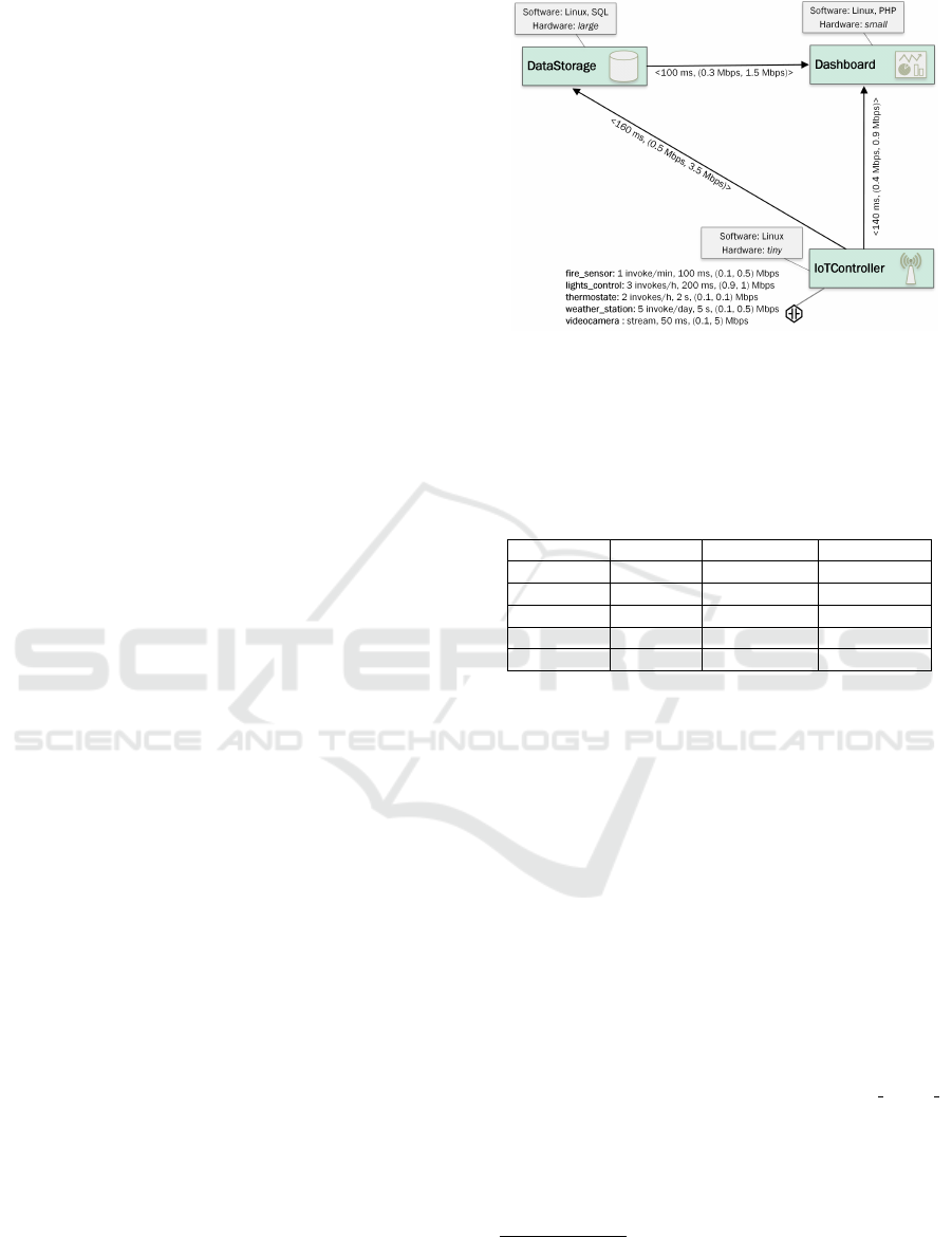
Consider a simple Fog application (Figure 1) that

manages ﬁre alarm, heating and A/C systems, inte-

rior lighting, and security cameras of a smart building.

The application consists of three microservices:

• IoTController, interacting with the connected cyber-

physical systems,

• DataStorage, storing all sensed information for fu-

ture use and employing machine learning tech-

niques to update sense-act rules at the IoTController

so to optimise heating and lighting management

based on previous experience and/or on people be-

haviour, and

• Dashboard, aggregating and visualising collected

data and videos, as well as allowing users to inter-

act with the system.

Each microservice represents an independently de-

ployable component of the application (Newman,

2015) and has hardware and software requirements in

order to function properly (as indicated in the grey

Figure 1: Fog application of the motivating example.

box associated with each component). Hardware re-

quirements are expressed in terms of the virtual ma-

chine (VM) types

listed in Table 1 and must be ful-

ﬁlled by the VM that will host the component.

Table 1: Hardware speciﬁcation for different VM types.

VM Type vCPUSs RAM (GB) HDD (GB)

tiny 1 1 10

small 1 2 20

medium 2 4 40

large 4 8 80

xlarge 8 16 160

App components must cooperate so that well-

deﬁned levels of service are met by the application.

Hence, communication links supporting component-

component interactions should provide suitable end-

to-end latency and bandwidth (e.g., the IoTController

should reach the DataStorage within 160 ms and have

at least 0.5 Mbps download and 3.5 Mbps upload free

bandwidth

). Component-Things interactions have

analogous constraints, and also specify the sampling

rate at which IoTController is expected to query Things

at runtime.

Figure 2 shows the infrastructure – two Cloud

data centres, three Fog nodes and nine Things – se-

lected by the system integrators in charge of deploy-

ing the smart building application for one of their cus-

tomers. The deployed application will have to exploit

the Things connected to Fog 1 and the weather station 3

at Fog 3. Furthermore, the customer owns Fog 2, what

makes deploying components to that node cost-free

for the system integrators.

All Fog and Cloud nodes are associated with pric-

ing schemes either to buy an instance of a certain

Adapted from OpenStack Mitaka ﬂavours:

https://docs.openstack.org/.

Arrows on the links in Figure 1 indicate the upload di-

rection.

Deploying Fog Applications: How Much Does It Cost, By the Way?

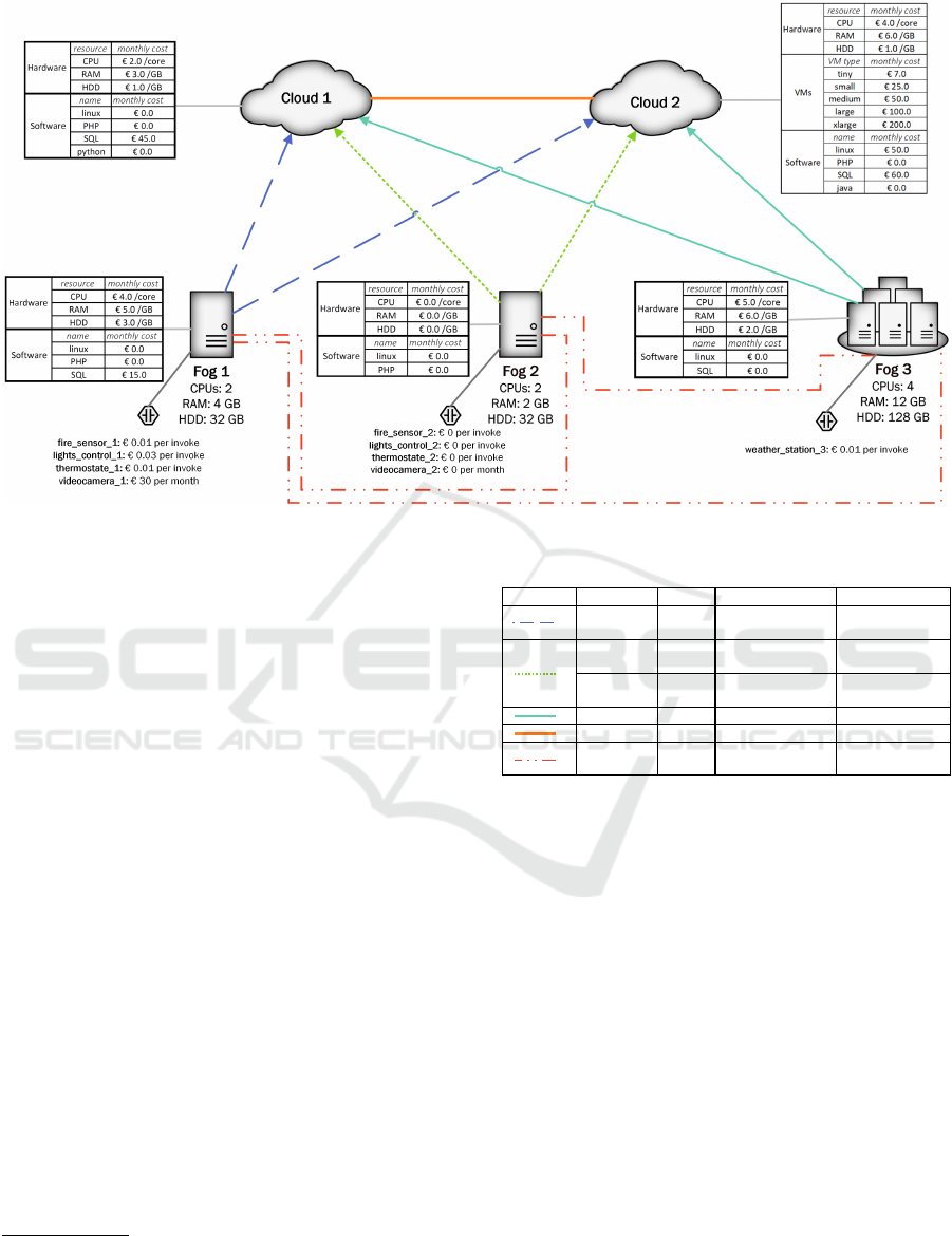
Figure 2: Fog infrastructure of the motivating example.

VM type (e.g., a tiny instance at Cloud 2 costs e 7 per

month), or to build on-demand instances by selecting

the required number of cores and the needed amount

of RAM and HDD to support a given component.

Fog nodes offer software capabilities, along with

limited hardware resources (i.e., RAM, HDD, CPUs).

Cloud nodes offer software capabilities, whilst hard-

ware is considered unbounded assuming that one can

always purchase extra or larger instances on-demand.

Finally, Table 2 lists the QoS proﬁles of the avail-

able communication links

, which are represented as

probability distributions based on real data

, to ac-

count for variations in the QoS they provide. Green

color links at Fog 2 initially feature a 3G Inter-

net access. As per the current technical proposals

(e.g., (Bonomi et al., 2014) and (OpenFog, 2016)),

we assume Fog and Cloud nodes being able to ac-

cess directly connected Things as well as Things at

neighbouring nodes via a speciﬁc middleware layer

(through the associated communication links).

Planning to sell the deployed solution for e 1,500

a month, the system integrators set the limit of the

monthly deployment cost at e 850. Also, the cus-

tomer requires the application to be compliant with

the speciﬁed QoS requirements at least 98% of the

time. Then, interesting questions for the system inte-

grators before the ﬁrst deployment of the application

Arrows on the links in Figure 2 indicate the upload di-

rection.

Satellite: https://www.eolo.it/, 3G/4G: https://www.

agcom.it, VDSL: http://www.vodafone.it.

Table 2: QoS proﬁles of communication links.

Dash Type Profile Latency Download Upload

3G 54 ms

99.6%: 9.61 Mbps

0.4%: 0 Mbps

99.6%: 2.89 Mbps

0.4%: 0 Mbps

4G 53 ms

99.3%: 22.67 Mbps

0.7%: 0 Mbps

99.4%: 16.97 Mbps

0.6%: 0 Mbps

VDSL 60 ms 60 Mbps 6 Mbps

Fibre 5 ms 1000 Mbps 1000 Mbps

WLAN 15 ms

90%: 32 Mbps

10%: 16 Mbps

90%: 32 Mbps

10%: 16 Mbps

98%: 4.5 Mbps

2%: 0 Mbps

Satellite 14M

40 ms

98%: 10.5 Mbps

2%: 0 Mbps

are, for instance:

Q1(a) — Is there any eligible deployment of the

application reaching the needed Things at Fog

1 and Fog 3, and meeting the ﬁnancial (at most

e 850 per month) and QoS-assurance (at least

98% of the time) constraints mentioned above?

Q1(b) — Which eligible deployments minimise

resource consumption in the Fog layer so to per-

mit future deployment of services and sales of vir-

tual instances to other customers?

Suppose that with an extra monthly investment of

e 20, system integrators can exploit a 4G connection

at Fog 2. Then:

Q2 — Would there be any deployment that com-

plies with all previous requirements and reduces

ﬁnancial cost and/or consumed Fog resources

when upgrading from 3G to 4G at Fog 2?

In Section 5, we will show how the new version of

FogTorchΠ – extended with the cost model of Section

CLOSER 2018 - 8th International Conference on Cloud Computing and Services Science

4 – can be exploited to obtain answers to all the above

questions.

3 OVERVIEW OF FogTorchΠ

FogTorchΠ (Brogi et al., 2017) is an open-source Java

prototype

that permits to describe IoT+Fog+Cloud

infrastructures and applications (based on the model

of (Brogi and Forti, 2017)) so to determine QoS- and

context-aware application deployments. Before in-

troducing the cost-aware extension to FogTorchΠ, we

summarise its basic functioning. FogTorchΠ inputs:

1. an IoT+Fog+Cloud infrastructure I, with the

speciﬁcation of the Fog and Cloud nodes available

for deployment (each with its hardware, software

and IoT capabilities), and the probability distri-

butions of the QoS (viz., latency, bandwidth) fea-

tured by the communication links interconnecting

such nodes

2. a multi-component application A, specifying all

hardware (i.e., CPU, RAM, storage), software

(i.e., OS, libraries, frameworks) and IoT require-

ments (i.e., which type of Things to exploit)

of each component, and the QoS (i.e., latency

and bandwidth) needed to support component-

component and component-Thing interactions,

3. a Things binding ϑ, mapping each IoT require-

ment of an application component to an actual

Thing in I, and

4. a deployment policy δ(γ), white-listing the nodes

where component γ of A can be deployed

accord-

ing to security or business-related constraints.

Based on such input, FogTorchΠ determines all the el-

igible deployments of the components of A to Cloud

or Fog nodes in I. An eligible deployment ∆ maps

each component γ of A to a Cloud or Fog node n

in I so that (1) n ∈ δ(γ) and it satisﬁes the process-

ing requirements of γ, (2) hardware resources are

enough to deploy all components of A mapped to

n, (3) Things speciﬁed in ϑ are reachable, and (4)

component-component and component-Thing inter-

actions mapped to the same communication link do

not exceed the available bandwidth and meet their la-

tency requirements.

Available at https://github.com/di-unipi-socc/Fog

TorchPI/tree/costmodel/.

Actual implementations in Fog landscapes can exploit

monitoring tools (e.g., (Breitbart et al., 2001), (Fatema

et al., 2014)) to get updated information on the state of I.

When δ is not speciﬁed for a component γ of A, γ can

be deployed to any compatible node in I.

1: procedure MONTECARLO(A, I, ϑ, δ, n)

2: D ←

0  dictionary of h∆, counteri

3: for n times do

4: I

← SAMPLELINKSQOS(I)

5: E ← FINDDEPLOYMENTS(A, I

, ϑ, δ)

6: D ← UNIONUPDATE(D, E)

7: end for

8: for ∆ ∈ keys(D) do

9: D[∆] ← D[∆]/n

10: end for

11: return D

12: end procedure

Figure 3: Pseudocode of the Monte Carlo simulation in Fog-

TorchΠ.

FogTorchΠ employs the Monte Carlo method

(Dunn and Shultis, 2011) to estimate the QoS-

assurance of output deployments, by aggregating the

eligible deployments obtained when varying the QoS

of communication links (as per their input probabil-

ity distributions). In addition, FogTorchΠ outputs the

percentage of resources (RAM and HDD) consumed

in the Fog layer (or in speciﬁed Fog nodes) after per-

forming an eligible deployment.

Figure 3 shows the pseudocode of FogTorchΠ func-

tioning. First, an empty dictionary D is created to

contain key-value pairs h∆,counteri, where the key

(∆) represents an eligible deployment and the value

(counter) keeps track of how many times ∆ will be

generated during the Monte Carlo simulation (line 2).

Then, at the beginning of each run of the simulation,

a state I

of the infrastructure is sampled according to

the probability distributions of the QoS of the com-

munication links in I (line 4).

The function FINDDEPLOYMENTS(A, I

, ϑ, δ)

(line 5) employs an exhaustive (backtracking) search

to determine the set E of eligible deployments ∆ of A

to I

, i.e. deployments of A that satisfy all processing

and QoS requirements in that particular state of the

infrastructure. Each output deployment ∆ also con-

tains information about its Fog resource consumption,

which is computed during the search. The objective of

this step is to look for eligible deployments, whilst dy-

namically simulating changes in the underlying net-

work conditions. At the end of each run, the set E of

eligible deployments of A to I

is used to update D.

The function UNIONUPDATE(D, E) (line 6) updates

D by adding deployments h∆, 1i discovered during the

last run (∆ ∈ E \ keys(D)) and by incrementing the

counter of those deployments that had already been

found in a previous run (∆ ∈ E ∩keys(D)).

At the end of the simulation (n ≥ 100,000), the

QoS-assurance of each deployment ∆ ∈ keys(D) is

computed by dividing the counter associated to ∆ by

n (lines 8–10). Thus, the QoS-assurance is the per-

centage of runs a certain deployment ∆ was found by

Deploying Fog Applications: How Much Does It Cost, By the Way?

FINDDEPLOYMENTS(A, I

, ϑ, δ). Such percentage

estimates how likely ∆ is to meet all QoS constraints

of A, taking into account variations in the communi-

cation links as per historical behaviour of I. Finally,

dictionary D is returned (line 11).

The next section introduces the cost model ex-

tension of FogTorchΠ, which permits estimating the

monthly deployment cost of output deployments. We

extended FINDDEPLOYMENTS(A, I

, ϑ, δ) so to re-

turn each deployment ∆ with its associated monthly

cost

in addition to its Fog resource consumption.

4 COST MODEL

Our cost model extends to Fog computing previous

efforts in Cloud VM cost modelling (D

ıaz et al.,

2017), and includes software costs, and costs due to

IoT (Niyato et al., 2016).

At any Cloud or Fog node n, our cost model con-

siders that a hardware offering H can be either de-

fault VMs (Table 1) offered at a ﬁxed monthly fee

or on-demand VMs (built with an arbitrary amount

of cores, RAM and HDD). Being R the set of re-

sources considered when building on-demand VMs

(viz., R = {CPU,RAM,HDD}), the estimated monthly

cost for a hardware offering H at node n is

p(H,n) =







c(H,n) if H is a default VM

∑

ρ∈R

[H.ρ × c(ρ,n)] if H is an on-demand VM

where c(H,n) is the monthly cost of a default VM

H at Fog or Cloud node n, whilst H.ρ indicates the

amount of resource ρ ∈ R used by

the on-demand

VM represented by H, and c(ρ,n) is the unit monthly

cost at n for resource ρ.

Analogously, for any given Cloud or Fog node n,

a software offering S can be either a predetermined

software bundle or an on-demand subset of the soft-

ware capabilities available at n (each sold separately).

The estimated monthly cost for S at node n is

p(S,n) =

(

c(S,n) if S is a bundle

∑

s∈S

c(s,n) if S is on-demand

Cost computation is performed on-the-ﬂy during the

search step, envisioning the possibility to exploit cost as a

heuristic to lead the search algorithm towards a best candi-

date deployment.

Bounded by the maximum amount purchasable at any

chosen Cloud or Fog node.

where c(S, n) is the price for the software bundle S

at node n, and c(s,n) is the monthly cost of a single

software s at n.

Finally, in Sensing-as-a-Service (Perera, 2017)

scenarios, a Thing offering T exploiting an actual

Thing t can be offered at a monthly subscription fee

or through a pay-per-invocation mechanism. Then,

the cost for offering T at Thing t is

p(T,t) =

(

c(T,t) if T is subscription based

T.k × c(t) if T is pay-per-invocation

where c(T,t) is the monthly subscription fee for T at

t, while T.k is the number of monthly invocations ex-

pected over t and c(t) is the cost per invocation at t

(including Thing usage and/or data transfer costs).

In what follows, we assume that ∆ is an eligible

deployment for an application A to an infrastructure

I, as introduced in Section 3. In addition, let γ ∈ A

be a component of the considered application A, and

let γ.H , γ.Σ and γ.Θ be its hardware, software and

Things requirements, respectively. Overall, the ex-

pected monthly cost for a given deployment ∆ can be

ﬁrst approximated by combining the previous pricing

schemes as in:

cost(∆,ϑ,A) =

∑

γ∈A

p(γ.H ,∆(γ)) + p(γ.Σ, ∆(γ)) +

∑

r∈γ.Θ

p(r,ϑ(r))

Although this formula gives an estimate of the

monthly cost for a given deployment, yet it does not

feature a way to select the “best” offering to match

the application requirements at the VM, software and

IoT levels. Particularly, it may lead the choice always

to on-demand and pay-per-invocation offerings when

the application requirements do not match exactly de-

fault or bundled offerings, or when a Cloud provider

does not offer a particular VM type (e.g., starting its

offerings from medium). This can lead to overesti-

mate the monthly deployment cost.

For instance, consider the infrastructure of Fig-

ure 2 and the hardware requirements of a compo-

nent to be deployed to Cloud 2, speciﬁed as R =

{CPU : 1,RAM : 1GB,HDD : 20GB}. Since no exact match-

ing between the requirement and an offering at Cloud

2 exists, this ﬁrst cost model would select an on-

demand instance, and estimate its cost of e 30

However, Cloud 2 also provides a small instance that

can satisfy the requirements at a (lower) cost of e 25.

Since larger VM types always satisfy smaller

hardware requirements, bundled software offerings

may satisfy multiple software requirements at a lower

price, and subscription-based Thing offerings can be

e 30 = 1 CPU x e 4/core + 1 GB RAM x e 6/GB + 20 GB HDD x e 1/GB

CLOSER 2018 - 8th International Conference on Cloud Computing and Services Science

more or less convenient depending on the number

of invocations on a given Thing, some policy must

be used to choose the “best” offerings for each soft-

ware, hardware and Thing requirement of an applica-

tion component. In what follows, we reﬁne our cost

model to also account for this fact.

A requirement-to-offering matching policy

(r, n) matches hardware or software requirements

r of a component (r ∈ {γ.H ,γ.Σ}) to the estimated

monthly cost of the offering that will support them

at Cloud or Fog node n, and a Thing requirement

r ∈ γ.Θ to the estimated monthly cost of the offering

that will support r at Thing t.

Overall, this reﬁned version of the cost model

permits to estimate the monthly cost of ∆ including

a cost-aware matching between application require-

ments and infrastructure offering (for hardware, soft-

ware and IoT), chosen as per p

. Hence:

cost(∆,ϑ,A) =

∑

γ∈A

(γ.H ,∆(γ)) + p

(γ.Σ,∆(γ)) +

∑

r∈γ.Θ

(r,ϑ(r))

The new version of FogTorchΠ – extended with the

cost model – exploits a best-ﬁt lowest-cost policy for

choosing hardware, software and Thing offerings. In-

deed, it selects the cheapest between the ﬁrst default

VM (from tiny to xlarge) that can support γ.H at node

n and the on-demand offering built as per γ.H . Like-

wise, software requirements in γ.Σ are matched with

the cheapest compatible version available at n, and

Thing per invocation offer is compared to monthly

subscription so to select the cheapest

Formally, the cost model used by the new version

of FogTorchΠ can be expressed as:

(H ,n) = min{p(H,n)}

∀ H ∈ {default VMs, on-demand VM} ∧ H |= H

(Σ,n) = min{p(S,n)}

∀ S ∈ {on-demand, bundle} ∧ S |= Σ

(r,t) = min{p(T,t)}

∀ T ∈ {subscription, pay-per-invocation} ∧ T |= r

where O |= R reads as offering O satisﬁes require-

ments R.

It is worth noting that the proposed cost model

separates the cost of purchasing VMs from the cost of

purchasing software. This choice keeps the modelling

general enough to include both IaaS and PaaS Cloud

offerings. Furthermore, even if we referred to VMs as

the only deployment unit for application components,

Other policies are also possible such as, for instance,

selecting the largest offering that can accommodate a com-

ponent, or always increasing the component’s requirements

by some percentage (e.g., 10%) before selecting the match-

ing.

the model can be easily extended so to include other

types of virtual instances (e.g., containers).

5 MOTIVATING EXAMPLE

(CONTINUED)

We now present the results of running the new ver-

sion of FogTorchΠ over the smart building example

of Section 2 and to get answers for the questions of

the system integrators. FogTorchΠ outputs the eligible

deployments (as per Section 3) along with their esti-

mated QoS-assurance, Fog resource consumption and

monthly cost (as per Section 4).

Table 3: Eligible deployments generated by FogTorchΠ for

Q1 and Q2

Dep. ID IoTController DataStorage Dashboard

∆1 Fog 2 Fog 3 Cloud 2

∆2 Fog 2 Fog 3 Cloud 1

∆3 Fog 3 Fog 3 Cloud 1

∆4 Fog 2 Fog 3 Fog 1

∆5 Fog 1 Fog 3 Cloud 1

∆6 Fog 3 Fog 3 Cloud 2

∆7 Fog 3 Fog 3 Fog 2

∆8 Fog 3 Fog 3 Fog 1

∆9 Fog 1 Fog 3 Cloud 2

∆10 Fog 1 Fog 3 Fog 2

∆11 Fog 1 Fog 3 Fog 1

∆12 Fog 2 Cloud 2 Fog 1

∆13 Fog 2 Cloud 2 Cloud 1

∆14 Fog 2 Cloud 2 Cloud 2

∆15 Fog 2 Cloud 1 Cloud 2

∆16 Fog 2 Cloud 1 Cloud 1

∆17 Fog 2 Cloud 1 Fog 1

For question Q1(a), the new version of FogTorchΠ

outputs eleven eligible deployments (∆1 — ∆11 in Ta-

ble 3), determined as described in Section 3.

It is worth recalling that we envision remote access

to Things connected to Fog nodes from other Cloud

and Fog nodes. In fact, some output deployments

map components to nodes that do not direclty con-

nect to all the required Things. For instance, in

the case of ∆1, IoTController is deployed to Fog 2

but the required Things (ﬁre sensor 1, light control 1,

thermostate 1, video camera 1, weather station 3) are at-

tached to Fog 1 and Fog 3, still being reachable with

suitable latency and bandwidth.

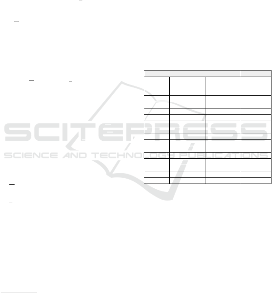
Figure 4 only shows the ﬁve output deployments

that satisfy the QoS and budget constraints imposed

Results and Python code to generate 3D plots as in

Figures 4 and 5 are available at: https://github.com/di-unipi-

socc/FogTorchPI/tree/costmodel/results/SMARTBUILDIN

G18/.

Deploying Fog Applications: How Much Does It Cost, By the Way?

by the system integrators. ∆3, ∆4, ∆7 and ∆10 all fea-

ture 100% QoS-assurance. Among them, ∆7 is the

cheapest in terms of cost, consuming as much Fog re-

sources as ∆4 and ∆10, although more with respect

to ∆3. On the other hand, ∆2, still showing QoS-

assurance above 98% and consuming as much Fog

resources as ∆3, can be a good compromise at the

cheapest monthly cost of e 800 (what answers ques-

tion Q1(b)).

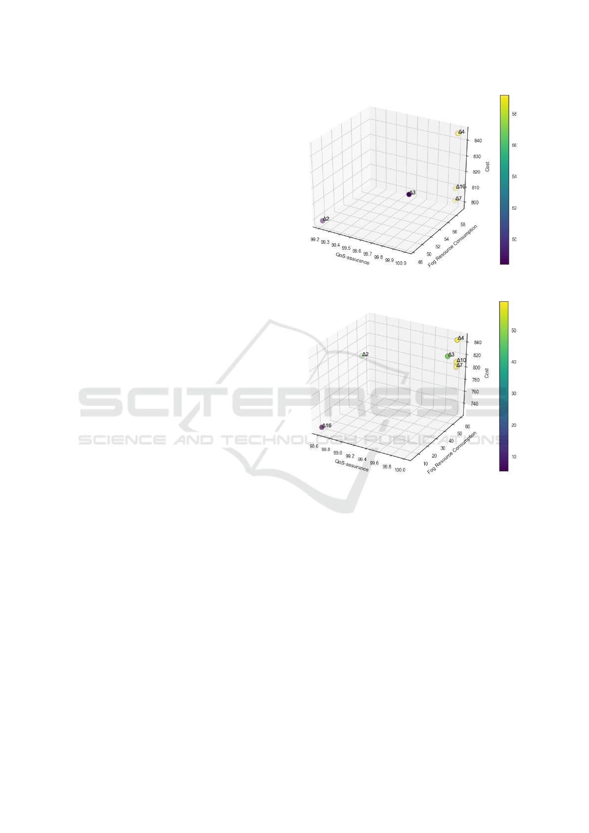
Finally, to answer question Q2, we change the In-

ternet access at Fog 2 from 3G to 4G. As mentioned

in Section 2, this increases the monthly expenses by

e 20. Running FogTorchΠ now reveals six new eli-

gible deployments (∆12 — ∆17) in addition to the

previous output. Among those, only ∆16 turns out

to meet also the QoS and budget constraints that the

system integrators require (Figure 5). Interestingly,

∆16 costs e 70 less than the best candidate for Q1(b)

(∆2), whilst sensibly reducing Fog resource consump-

tion. Hence, overall, the change from 3G to 4G would

lead to an estimated monthly saving of e 50, enacting

∆16 instead of ∆2.

The ﬁnal choice for a particular deployment is left

to the system integrators, leaving them the freedom

to select the “best” trade-off among QoS-assurance,

resource consumption and cost. Indeed, the analy-

sis of application speciﬁc requirements (along with

data on infrastructure behaviour) can lead decision to-

wards different segmentations of an application from

the IoT to the Cloud. Conversely to multi-objective

optimisation techniques (Gao et al., 2013), we fol-

low a human-driven approach – aided by predictive

tools like FogTorchΠ – to determine the best trade-off

among metrics that describe likely run time behaviour

of a deployment and make it possible to evaluate

changes in the infrastructure (or in the application)

before their actual implementation (what-if analyses

(Rizzi, 2009)).

6 RELATED WORK

With respect to the Cloud paradigm, the Fog intro-

duces new problems, mainly due to its pervasive geo-

distribution and heterogeneity, need for connection-

awareness, dynamicity and support to interactions

with the IoT, that were not taken into account by pre-

vious works (Varshney and Simmhan, 2017) (Wen

et al., 2017) (Arcangeli et al., 2015). Particularly,

some efforts in Cloud computing considered non-

functional requirements (e.g., (Nathuji et al., 2010),

(Cucinotta and Anastasi, 2011),(Rimal et al., 2011)

and (Durao et al., 2014)) or uncertainty of execu-

tion (as in Fog nodes) and security risks among in-

Figure 4: Results for Q1(a) and Q1(b). Colormap refers to

Fog resource consumption.

Figure 5: Results for Q2. Colormap refers to Fog resource

consumption.

teractive and interdependent components (Wen et al.,

2016). Only recently, (Wang et al., 2016) has linked

services and networks QoS by proposing a QoS-

and connection-aware Cloud service composition ap-

proach to satisfy end-to-end QoS requirements in the

Cloud.

To the best of our knowledge, few approaches

have been proposed so far to speciﬁcally model Fog

infrastructures and applications, as well as to deter-

mine and compare eligible deployments for an appli-

cation to an Fog infrastructure under different met-

rics. (Sarkar and Misra, 2016) aims at evaluating

service latency and energy consumption of the new

Fog paradigm applied to the IoT, as compared to tra-

ditional Cloud scenarios. The model of (Sarkar and

Misra, 2016), however, deals only with the behaviour

of software already deployed over Fog infrastructures

and simulates it mathematically.

CLOSER 2018 - 8th International Conference on Cloud Computing and Services Science

iFogSim (Gupta et al., 2017) is among the most

promising prototypes to simulate resource manage-

ment and scheduling policies applicable to Fog envi-

ronments with respect to their impact on latency, en-

ergy consumption and operational cost. The focus of

iFogSim model is mainly on stream-processing appli-

cations and hierarchical tree-like infrastructures, to be

mapped either Cloud-only or Edge-ward so to com-

pare results.

Building on top of iFogSim, (Bittencourt et al.,

2017) compares different task scheduling policies,

taking into account user mobility, optimal Fog re-

source utilisation and response time. (T

arneberg

et al., 2017) presents a distributed approach to cost-

effective application placement, at varying workload

conditions, with the objective of optimising opera-

tional cost across the entire infrastructure. Apropos,

(Shekhar et al., 2017) introduces a hierarchy-based

technique to dynamically manage and migrate appli-

cations between Cloud and Fog nodes. They exploit

message passing among local and global node man-

agers to guarantee QoS and cost constraints are met.

Similarly, (Skarlat et al., 2017) leverages the concept

of Fog colonies (Skarlat et al., 2016) for schedul-

ing tasks to Fog infrastructures, whilst minimising re-

sponse times. (Aazam et al., 2016) provides a ﬁrst

methodology for probabilistic record-based resource

estimation to mitigate resource underutilisation, to en-

hance the QoS of provisioned IoT services.

All the aforementioned approaches focus on

monolithic or DAG application topologies, and do

not take into account QoS for the interactions with

the IoT, nor historical data about Fog infrastructure

or deployment behaviour. Our approach permits in-

stead to express arbitrary multi-component applica-

tion topologies, as the one of the illustrated exam-

ple. Furthermore, the attempts to explicitly target and

support with predictive methodologies the decision-

making process to deploy IoT applications to the

Fog were very limited, and none of them considered

matching of application components to the best vir-

tual instance (Virtual Machine or container), depend-

ing on expressed preferences (e.g., cost or energy tar-

gets) in this work.

Pricing models for the Cloud are quite established

(e.g., (D

ıaz et al., 2017), (Niyato et al., 2016) and

references therein) but they do not account for costs

generated by the exploitation of IoT devices. Cloud

pricing models are generally divided into two types,

pay per use scheme and subscription-based. In (D

ıaz

et al., 2017), based on given user workload require-

ments, a Cloud broker chooses a best VM instance(s)

among several cloud providers. The total cost of de-

ployment is calculated considering hardware require-

ments such as number of CPU cores, VM types, time

duration, type of instance (reserved or pre-emptible),

etc.

On the other hand, IoT providers normally pro-

cess the sensory data coming from the IoT devices

and sell the processed information as value added ser-

vice to the users. (Niyato et al., 2016) shows how

they can also act as brokers, acquiring data from dif-

ferent owners and selling bundles. The authors of

(Niyato et al., 2016) also consider the fact that dif-

ferent IoT providers can federate their services and

create new offers for their end-users. Such end-

users are then empowered to estimate the total cost

of using IoT services by comparing pay-per-use and

subscription-based offers, depending upon their data

demand. In Fog scenario, however, there is a need

to compute IoT costs at a ﬁner level, also accounting

for data-transfer costs (i.e., event-based). More re-

cently, (Markus et al., 2017) propose a cost model for

IoT+Cloud scenario. Considering parameters such as

the type and number of sensors, number of data re-

quest and uptime of VM, their cost model can esti-

mate the cost of running an application over a certain

period of time.

Other recent studies tackle akin challenges from

an infrastructural perspective either focusing on scal-

able algorithms for QoS-aware placement of micro-

data centres (Selimi et al., 2017), on optimal place-

ment of data and storage nodes that ensures low la-

tencies and maximum throughput, optimising costs

(Naas et al., 2017), or on the exploitation of genetic

algorithms to place intelligent access points at the

edge of the network (Majd et al., 2017).

To the best of our knowledge, our attempt to

model costs in the Fog scenario is the ﬁrst that extends

Cloud pricing schemes to the Fog layer and integrates

them with costs that are typical of IoT deployments.

7 CONCLUDING REMARKS

In this paper, we presented a novel cost model to esti-

mate multi-component application deployment cost to

IoT+Fog+Cloud infrastructures. The model considers

various cost parameters (hardware, software and IoT),

extending Cloud computing cost models to the Fog

computing paradigm, whilst taking into account costs

associated to the usage of IoT devices and services.

We included it in the FogTorchΠ prototype to show

how it can assist IT experts in deciding how to dis-

tribute a multi-component application over a given in-

frastructures in a QoS-, context-, and cost-aware man-

ner. We envision the possibility of exploiting such a

cost model to drive design of billing of new services

Deploying Fog Applications: How Much Does It Cost, By the Way?

offered by small and medium enterprises in the Fog

marketplace. Indeed, supporting deployment decision

in the Fog requires comparing a multitude of offerings

where providers are able to deploy their applications

to their infrastructure integrated with the Cloud, with

the IoT, with federated Fog devices as well as with

user-managed devices.

We see three main directions for future work:

- Exploiting a multitude of highly distributed

nodes, Fog computing is likely to consume more

energy with respect to the Cloud. Application de-

ployments should also consider energy-related is-

sues so to guarantee reliable service provisioning

and longer deployment lifetime when exploiting

battery powered IoT devices or Fog nodes. Hence,

we aim at further extending our contribution to

consider energy consumption as a characterising

metric for eligible deployments.

- Monte Carlo simulation is in general computa-

tionally expensive but it can be efﬁciently par-

allelised and optimised. Furthermore, FogTorchΠ

exploits exponential search algorithms. Apropos,

another direction for future work is to parallelise

the simulation and tame the complexity of Fog-

TorchΠ algorithms to scale better over large infras-

tructures, by leading search with improved heuris-

tics and by approximating metrics estimation.

- Currently, Fog computing lacks medium to large

scale test-bed deployments (i.e., infrastructure

and applications) to test devised approaches. Last,

but not least, we intend to contribute further in en-

gineering FogTorchΠ and to assess validity of the

prototype over an experimental lifelike test-bed

that is currently at study.

REFERENCES

Aazam, M., St-Hilaire, M., Lung, C. H., and Lambadaris,

I. (2016). MeFoRE: QoE based resource estimation

at Fog to enhance QoS in IoT. In 2016 23rd In-

ternational Conference on Telecommunications (ICT),

pages 1–5.

Arcangeli, J.-P., Boujbel, R., and Leriche, S. (2015). Au-

tomatic deployment of distributed software systems:

Deﬁnitions and state of the art. Journal of Systems

and Software, 103:198–218.

Bittencourt, L. F., Diaz-Montes, J., Buyya, R., Rana, O. F.,

and Parashar, M. (2017). Mobility-aware Application

Scheduling in Fog Computing. IEEE Cloud Comput-

ing, 4(2):26–35.

Bonomi, F., Milito, R., Natarajan, P., and Zhu, J. (2014).

Fog computing: A Platform for Internet of Things

and Analytics. In Big Data and Internet of Things:

A Roadmap for Smart Environments, pages 169–186.

Breitbart, Y., Chan, C.-Y., Garofalakis, M., Rastogi, R.,

and Silberschatz, A. (2001). Efﬁciently monitoring

bandwidth and latency in IP networks. In INFOCOM

2001. Twentieth Annual Joint Conference of the IEEE

Computer and Communications Societies. Proceed-

ings. IEEE, volume 2, pages 933–942. IEEE.

Brogi, A. and Forti, S. (2017). QoS-aware Deployment of

IoT Applications Through the Fog. IEEE Internet of

Things Journal, 4(5):1185–1192.

Brogi, A., Forti, S., and Ibrahim, A. (2017). How to best

deploy your Fog applications, probably. In Rana, O.,

Buyya, R., and Anjum, A., editors, Proceedings of

1st IEEE International Conference on Fog and Edge

Computing (ICFEC), Madrid, pages 105–114.

Chiang, M. and Zhang, T. (2016). Fog and IoT: An

overview of research opportunities. IEEE Internet of

Things Journal, 3(6):854–864.

Cucinotta, T. and Anastasi, G. F. (2011). A heuristic

for optimum allocation of real-time service work-

ﬂows. In Service-Oriented Computing and Applica-

tions (SOCA), 2011 IEEE Int. Conf. on, pages 1–4.

IEEE.

Dastjerdi, A. V. and Buyya, R. (2016). Fog Computing:

Helping the Internet of Things Realize its Potential.

Computer, 49(8):112–116.

ıaz, J. L., Entrialgo, J., Garc

ıa, M., Garc

ıa, J., and Garc

ıa,

D. F. (2017). Optimal allocation of virtual machines

in multi-cloud environments with reserved and on-

demand pricing. Future Generation Computer Sys-

tems, 71:129–144.

Dunn, W. L. and Shultis, J. K. (2011). Exploring Monte

Carlo Methods. Elsevier.

Durao, F., Carvalho, J. F. S., Fonseka, A., and Garcia, V. C.

(2014). A systematic review on cloud computing. The

Journal of Supercomputing, 68(3):1321–1346.

Fatema, K., Emeakaroha, V. C., Healy, P. D., Morrison, J. P.,

and Lynn, T. (2014). A survey of Cloud monitoring

tools: Taxonomy, capabilities and objectives. Journal

of Parallel and Distributed Computing, 74(10):2918–

2933.

Gao, Y., Guan, H., Qi, Z., Hou, Y., and Liu, L. (2013). A

multi-objective ant colony system algorithm for vir-

tual machine placement in cloud computing. Journal

of Computer and System Sciences, 79(8):1230–1242.

Gupta, H., Dastjerdi, A. V., Ghosh, S. K., and Buyya,

R. (2017). iFogSim: A Toolkit for Modeling and

Simulation of Resource Management Techniques in

Internet of Things, Edge and Fog Computing En-

vironments. Software: Practice and Experience,

47(9):1275–1296.

Iorga, M. et al. (2017). The NIST Deﬁnition of Fog Com-

puting (draft SP 800-191).

Majd, A., Sahebi, G., Daneshtalab, M., Plosila, J., and Ten-

hunen, H. (2017). Hierarchal Placement of Smart

Mobile Access Points in Wireless Sensor Networks

Using Fog Computing. In 2017 25th Euromicro In-

ternational Conference on Parallel, Distributed and

Network-based Processing (PDP), pages 176–180.

Markus, A., Kertesz, A., and Kecskemeti, G. (2017). Cost-

CLOSER 2018 - 8th International Conference on Cloud Computing and Services Science

Aware Iot Extension of DISSECT-CF. Future Inter-

net, 9(3).

Naas, I., Raipin, P., Boukhobza, J., and Lemarchand, L.

(2017). iFogStor: an IoT Data Placement Strategy

for Fog Infrastructure. In Rana, O., Buyya, R., and

Anjum, A., editors, Proceedings of 1st IEEE Inter-

national Conference on Fog and Edge Computing,

Madrid. In press.

Nathuji, R., Kansal, A., and Ghaffarkhah, A. (2010). Q-

Clouds: Managing Performance Interference Effects

for QoS-Aware Clouds. Association for Computing

Machinery, Inc.

Newman, S. (2015). Building microservices: designing

ﬁne-grained systems. ” O’Reilly Media, Inc.”.

Niyato, D., Hoang, D. T., Luong, N. C., Wang, P., Kim,

D. I., and Han, Z. (2016). Smart data pricing mod-

els for the internet of things: a bundling strategy ap-

proach. IEEE Network, 30(2):18–25.

OpenFog (2016). OpenFog Reference Architecture.

Perera, C. (2017). Sensing as a Service for Internet of

Things: A Roadmap. Lulu. com.

Rimal, B. P., Jukan, A., Katsaros, D., and Goeleven,

Y. (2011). Architectural Requirements for Cloud

Computing Systems: An Enterprise Cloud Approach.

Journal of Grid Computing, 9(1):3–26.

Rizzi, S. (2009). What-if analysis. In Encyclopedia of

Database Systems, pages 3525–3529. Springer.

Sarkar, S. and Misra, S. (2016). Theoretical modelling of

fog computing: a green computing paradigm to sup-

port IoT applications. IET Networks, 5(2):23–29.

Selimi, M., Cerd

a-Alabern, L., S

anchez-Artigas, M., Fre-

itag, F., and Veiga, L. (2017). Practical Service Place-

ment Approach for Microservices Architecture.

Shekhar, S., Chhokra, A., Bhattacharjee, A., Aupy, G.,

and Gokhale, A. (2017). INDICES: Exploiting Edge

Resources for Performance-aware Cloud-hosted Ser-

vices. In Rana, O., Buyya, R., and Anjum, A., editors,

Proceedings of 1st IEEE International Conference on

Fog and Edge Computing, Madrid.

Skarlat, O., Nardelli, M., Schulte, S., and Dustdar, S.

(2017). Towards QoS-aware fog service placement.

In Rana, O., Buyya, R., and Anjum, A., editors, Pro-

ceedings of 1st IEEE International Conference on Fog

and Edge Computing, Madrid. In press.

Skarlat, O., Schulte, S., Borkowski, M., and Leitner, P.

(2016). Resource Provisioning for IoT Services in the

Fog. In SOCA, pages 32–39. IEEE.

arneberg, W., Papadopoulos Vittorio, A., Mehta, A.,

Tordsson, J., and Kihl, M. (2017). Distributed Ap-

proach to the Holistic Resource Management of a Mo-

bile Cloud Network. In Rana, O., Buyya, R., and

Anjum, A., editors, Proceedings of 1st IEEE Inter-

national Conference on Fog and Edge Computing,

Madrid.

Varshney, P. and Simmhan, Y. (2017). Demystifying Fog

Computing: Characterizing Architectures, Applica-

tions and Abstractions. In 2017 IEEE 1st Inter-

national Conference on Fog and Edge Computing

(ICFEC), pages 115–124.

Wang, S., Zhou, A., Yang, F., and Chang, R. N. (2016).

Towards Network-Aware Service Composition in the

Cloud. IEEE Transactions on Cloud Computing.

Wen, Z., Cala, J., Watson, P., and Romanovsky, A. (2016).

Cost effective, reliable and secure workﬂow deploy-

ment over federated clouds. IEEE Transactions on

Services Computing, PP(99):1–1.

Wen, Z., Yang, R., Garraghan, P., Lin, T., Xu, J., and Rovat-

sos, M. (2017). Fog Orchestration for Internet of

Things Services. IEEE Internet Computing, 21(2):16–

24.

Deploying Fog Applications: How Much Does It Cost, By the Way?