Detecting Anomalies in Device Event Data in the IoT

Irene Cramer, Prakash Govindarajan, Minu Martin, Alexandr Savinov,

Arun Shekhawat, Alexander Staerk and Appasamy Thirugnana

Bosch Software Innovations GmbH, IoT Analytics, Ullsteinstraße 128, 12109 Berlin, Germany

Keywords: Internet of Things, Anomaly Detection, Analytics, Data Mining, Big Data, Cloud Computing.

Abstract: This paper describes an approach to detecting anomalous behavior of devices by analyzing their event data.

Devices from a fleet are supposed to be connected to the Internet by sending log data to the server. The task

is to analyze this data by automatically detecting unusual behavioral patterns. Another goal is to provide

analysis templates that are easy to customize and that can be applied to many different use cases as well as

data sets. For anomaly detection, this log data passes through three stages of processing: feature generation,

feature aggregation, and analysis. It has been implemented as a cloud service which exposes its functionality

via REST API. The core functions are implemented in a workflow engine which makes it easy to describe

these three stages of data processing. The developed cloud service also provides a user interface for visualizing

anomalies. The system was tested on several real data sets, such as data generated by autonomous lawn

mowers where it produced meaningful results by using the standard template and only little parameters.

1 INTRODUCTION

Today, connected devices in the Internet of Things

(IoT) generate more data than social networks. A

device can send data several times per second and

with millions of connected devices, a typical data

processing platform might need to deal with billions

of such incoming events a day. Even though

processing this amount of data is obviously a highly

non-trivial technological challenge, it is clear that the

device data itself is not actionable per se. In order to

derive actionable insights, the collected data has to be

analyzed.

One important task that can be effectively solved

by means of data analysis is anomaly detection which

“refers to the problem of finding patterns in data that

do not conform to expected behavior” (Chandola et

al., 2009). Its goal is to find devices with behavior that

significantly differs from what is expected or has

been observed before.

There are many different types of anomalies and

many different problem domains with their specific

data and problem formulations. In this paper, we limit

the scope of our research by the following

assumptions:

 [Asynchronous events] The data is sent

asynchronously and irregularly. Each event has

a time stamp but is not a regular time series.

This assumption means that it is essentially

impossible to directly analyze the device data

and therefore some pre-processing is required.

 [Device aware analysis] Events are sent by a

fleet consisting of thousands and millions of

different devices. In particular, “normal”

behavior is now a characteristic of the whole

fleet, however derived features have to be

computed and anomalies have to be detected

for individual devices.

 [Multivariate data] The events have many

properties and are not a univariate time series.

This means that it is not possible to use classic

statistical algorithms like ARIMA (Box &

Jenkins, 1976) which are known to be quite

effective for univariate numeric time series but

cannot be applied to our more complex use

cases.

 [Semi-structured data] Events can also contain

semi-structured data like JSON with nested

values. The events have both categorical and

numeric characteristics. In particular, it is quite

possible that devices do not send any numeric

characteristics at all. This immediately

excludes many traditional data analysis

algorithms.

Cramer, I., Govindarajan, P., Martin, M., Savinov, A., Shekhawat, A., Staerk, A. and Thirugnana, A.

Detecting Anomalies in Device Event Data in the IoT.

DOI: 10.5220/0006670100520062

In Proceedings of the 3rd International Conference on Internet of Things, Big Data and Security (IoTBDS 2018), pages 52-62

ISBN: 978-989-758-296-7

From the technological point of view, we have the

following design goals leading to the corresponding

challenges:

 [Analysis in the cloud] The developed

functionality has to be easily accessible in the

cloud. This assumption immediately excludes

many possible solutions based on stand-alone

analysis tools like Knime (Berthold et al.,

2007) and enterprise level technologies.

 [Easy to use] Our goal is to develop a

prototypical analysis workflow which can be

easily parameterized by specifying a limited set

of domain-specific parameters. It is opposed to

developing a full-featured system with dozens

or hundreds of parameters requiring high

expertise.

 [Extensibility and parameterization]

Frequently, the ease of use is achieved by

limiting the system functionality but this is

precisely what we want to avoid. Our goal is to

make it possible to provide various custom

extensions including user-defined functions

which are normally required for advanced and

domain-specific analysis scenarios.

In order to satisfy these design goals, we decided

to develop a general-purpose analysis template which

aims at anomaly detection. This template is

essentially an analysis workflow consisting of several

predefined data processing nodes. These nodes,

however, are supposed to be configured depending on

the concrete use case and data to be analyzed. In other

words, instead of exposing the complete functionality

of a general-purpose workflow engine (which is

difficult to use and parameterize) and building a

completely predefined analysis scenario, we chose an

intermediate solution which is, on one hand, simple

enough, and on the other hand, provides high

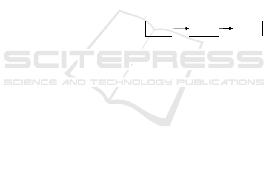
flexibility. This data analysis template consists of the

following steps (Fig. 1):

 [Feature generation] Raw data might not be

appropriate for analysis. The goal of this step is

to define new domain-specific features which

are better indicators of possible anomalies.

Each individual feature is implemented as a

user-defined function in Python.

 [Data aggregation] Raw data may have the

form of irregular events generated by devices.

The goal of this step is to convert sequences of

asynchronous events into regular time series.

First, all events for each individual device are

grouped by specifying an interval length, for

example, 1 hour or 1 minute. Then the event

properties are aggregated by applying either

standard (like mean or variance) or

user-defined aggregate functions in Python.

 [Data analysis] The main task of this

component is to detect anomalies in the

pre-processed data (generated by the previous

nodes) by applying data mining algorithms.

The analysis computes an anomaly score taking

values between 0 (no anomaly) and 1

(anomaly). The main challenge here is to

choose an appropriate data mining algorithm

and tune its parameters.

In order to implement these analysis steps, we

developed a general-purpose workflow engine in

Python by using such libraries as pandas and

scikit-learn. However, its full functionality is

not directly exposed to the user. Instead, its

workflows are preconfigured for certain

domain-specific tasks like anomaly detection or

predictive maintenance so that the user has to only

parameterize this template using an easy-to-use UI.

Figure 1: Analysis steps in anomaly detection.

The developed approach to anomaly detection

was tested on the following use case. Data is

produced by Bosch automatic lawn mowers (ALM)

sold under the brand name Indego. Indegos are

cordless devices which are operated by human

owners but work in an autonomous mode. Their task

is to mow the marked area by loading their batteries,

if necessary. Since they are connected to the internet,

they are sending various diagnostic messages to the

server.

Messages received from all devices are collected

as log files where one line is one message which

contains such standard fields as time stamp and

message id. Here is an example of fields from 3

messages:

status, {"state":519, "error":57}, null

get_map, {"state":6103, "error":504}, null

status, null, 37.0

These messages have one field in JSON format which

stores the current state of the device and error code.

There are also numeric fields like 37.0 which

represents the actual area that has been mowed. There

are much more parameters in these logs and most of

them are categorical values. The messages are sent

asynchronously at irregular intervals and not all fields

are present in all messages (there are many null

Feature

generation

Data

aggregation

Data analysis

Detecting Anomalies in Device Event Data in the IoT

values). The number of devices sending data is about

9,000. The analyzed data set contained messages sent

by these devices for one month. The size of this data

set was 3,919,908 lines and about 2.5 GB as a CSV

file. On average, each device was sending one log

message for about 3 minutes. The task is to monitor

their behavior by regularly analyzing these logs and

automatically detecting anomalies. The system

should identify a list of devices with the top anomaly

score. This list is then supposed to be manually

processed, for example, in the service center.

In this paper, we describe an approach to detecting

anomalies in event data in the IoT which has been

implemented as an Anomaly Detection Service

(ADS) running in the Bosch IoT Cloud

(BIC). The

paper makes two main contributions: 1) We introduce

general-purpose analysis templates which can be

easily parameterized and used for device-aware

anomaly detection by analyzing asynchronous

multivariate semi-structured data, and 2) we

implement this approach as a cloud service which can

be easily provisioned and used from within other

applications or services.

The paper is divided into the following sections.

Sections 2, 3, and 4 describe three main data

processing steps our analysis template consists of:

feature generation, data aggregation, and analysis.

Section 5 describes the implementation of this

approach as a cloud service and Section 6 makes

concluding remarks and provides a future outlook.

2 FEATURE GENERATION

2.1 Feature Engineering

Data preparation is a very important step in any data

analysis which significantly influences the quality of

the obtained results. In the overall analysis process,

various data pre-processing tasks can account for

most of the difficulties, and therefore choosing a

technology for efficient development and execution

of such scripts is of very high importance. This

process is frequently referred to as data wrangling

which is defined as “iterative data exploration and

transformation that enables analysis” (Kandel, 2011;

Savinov, 2014).

There are several major approaches to data pre-

processing and data wrangling which are shortly

listed below:

 Query-based approaches. All necessary data

transformations are performed by the

https://www.bosch-iot-suite.com/analytics/

underlying data management system using its

query language which is normally SQL.

 MapReduce-based approach. This approach is

based on two operations of Map and Reduce

which are implemented on top of a distributed

file system like Hadoop (Dean & Ghemawat,

2004) and Spark (Zaharia et al., 2012).

 Extract, Transform, Load (ETL). This

technology has been developed mainly for

pre-processing operational data and loading it

into a data warehouse.

These conventional approaches have two

important properties:

 [Dedicated system or framework] The

necessary transformations are performed

separately from the data analysis step.

 [Generating new sets or collections] The data

transformation procedure processes input sets

and produces an output set. It is a row-oriented

approach where rows can be represented as

tuples in a relational database, key-value pairs

in MapReduce or event objects in complex

event processing systems.

In contrast to these conventional approaches, our

feature generation module is focused on defining and

computing new domain-specific features, that is, one

feature is a unit of definition in the data

transformation model. The goal of domain-specific

features is to increase the level of abstractions and to

encode significant portions of domain knowledge and

problem semantics. The ability to define such features

determines how successful the data analysis process

will be (Guyon et al., 2006). This means that before a

data analysis algorithm can be applied to data, this

data has to be accordingly transformed and, what is

important, the result of this transformation determines

if the algorithm will find something interesting or not.

Since domain-specific features must contain a

significant portion of domain knowledge, they should

be produced in cooperation with a domain expert.

There can be, of course, many such features defined.

The main goal at this stage is to increase the semantic

level of available features so that it is easier for the

analysis algorithm to find anomalies. Domain experts

and data scientists produce features which explicitly

represent some partial and relatively simple

knowledge while the data mining algorithm increases

this level even higher by finding dependencies among

these (and original) features and representing them as

the final result. Essentially, feature engineering where

high level domain-specific features are defined by

domain experts can be viewed as an approach to deep

http://www.bosch-iot-cloud.com/

IoTBDS 2018 - 3rd International Conference on Internet of Things, Big Data and Security

learning which works even if not enough data is

available.

The analysis workflow engine that we have

developed is based on the following main

assumptions:

 Feature generation should be an integral part of

the whole data analysis process and, therefore

it has to be described and executed using the

same execution environment. In other words,

we do not want to separate data pre-processing

from other analysis steps because these steps

can be tightly connected and because such a

separation can limit the overall performance.

 Any new feature is a column and, hence the

main unit of definition and transformation is

that of a column. The task is then to describe

how new columns (features) are defined in

terms of other existing columns. For that

purpose, we have used a functional approach

where a unit of definition is a function. This

allows us to avoid explicit loops through the

data sets and define functions using other

functions. It is opposed to the conventional

approaches where new outputs are defined in

terms of input rows. The column-oriented data

representation is very popular in database

management systems (Abadi, 2007; Copeland

& Khoshafian, 1985) but it is less used in data

processing systems. Our implementation is

conceptually similar to the approach described

in Savinov, 2016.

 Although the functional approach is very

convenient for feature generation, there are

many tasks where it is necessary to process sets

and therefore set-operations should also be

supported. In our approach, one node of the

analysis workflow generates one set.

2.2 User-Defined Functions as Features

We have decided to use the Python pandas library

(McKinney, 2010; McKinney, 2011) as a basis for all

our data analysis functions including feature

generation. The main reason for choosing this

technology is that pandas provides the possibility to

easily integrate arbitrary user-defined functions into

the analysis workflow and the availability of a wide

range of standard data processing mechanisms and

analysis algorithms.

The main data structure in pandas is that of

DataFrame which is essentially a data table with

many data processing operations. The idea of our

approach to feature generation is that for a given table

with some columns, a new column is defined by

providing one Python function (called lambda in

functional programming). This function takes some

values as arguments and returns one output value.

Note that this function is unaware of the existence of

any tables or data rows—it transforms one or more

input values into one output value. Writing such

functions is known to be easy for ordinary users

because it is similar to normal arithmetic expressions.

In order to define a new column storing values of

a new feature, it is necessary to provide a Python

function as well as a name for this new column. The

system then will apply this function to all rows of the

input table and store the output values of this function

in the new column. Note that column definitions can

use existing columns as well as previously defined

columns. The computation of all new features in this

case can be represented as a graph of column

definitions where each next column is defined in

terms of some previous column.

For example, assume that a source event stores

inside and outside temperature. However, for

detecting anomalies their absolute values are not

important. It is rather important to know the

difference between them. In this case, it is necessary

to define a new derived feature which computes this

difference as the following Python function:

def temp_diff(row):

return row['inside'] - row['outside']

Here the row argument references the current row of

the table. Access to the fields is performed using an

array index with the column name.

In case a new feature depends on only one input

column, the syntax can be simplified and the input

argument represents directly the value of this column.

For example, the next feature will compare the

temperature difference with a fixed threshold:

def threshold_achieved(diff):

if diff > 30:

return 'high'

else:

return 'low'

Internally, the workflow engine written in Python

will collect all these definitions as user-defined

functions and then apply them to the input data frame.

This operation is executed as follows:

df['temp_diff'] = df.apply(temp_diff)

After all feature definitions have been computed, the

table with the new columns is returned and can be

used for the next steps of the data processing

workflow.

Derived features can, of course, be much more

complex and encode any domain-specific knowledge

Detecting Anomalies in Device Event Data in the IoT

about what is important for detecting anomalies. The

only limitation is that new features can be defined

only in terms of one data row—they cannot access

and use other rows for computing the output. This

limitation is overcome by the data aggregation node

described in the next section.

3 DATA AGGREGATION

3.1 Aggregation for Anomaly Detection

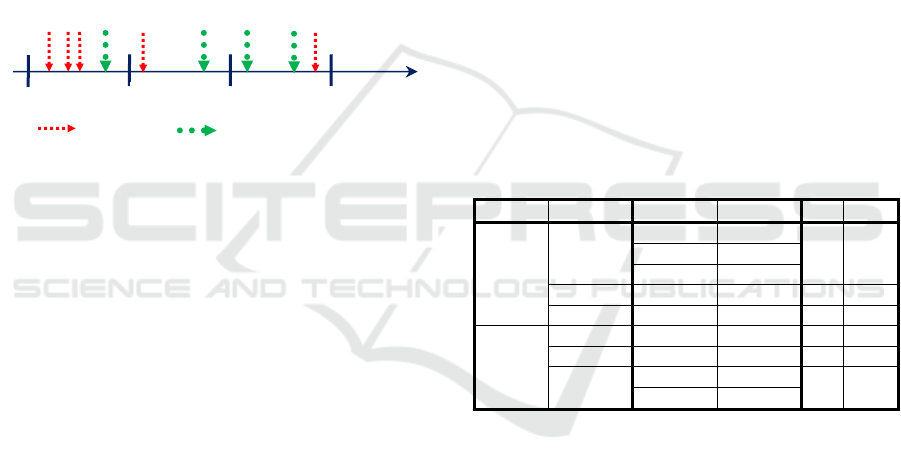
A typical sequence of device events is shown in Fig. 2

where events from different devices are represented

by different colors. Here we see that some intervals

have quite a lot of events while other intervals are

rather sparse.

Figure 2: Grouping events into fixed length time intervals.

Detecting anomalies where the state and behavior

of each device is represented as one event (point

anomaly) can be therefore rather difficult. The data

aggregation step in our anomaly detection approach

is aimed at solving the problems that arise from the

asynchronous nature of device data:

 [Producing time series] Many data analysis

algorithms are designed to process only regular

time series. Therefore, irregular event data has

to be aggregated and transformed into a time

series.

 [Down-sampling time series] Even if the input

data is a regular time series, it might be

necessary to downs-ample it. For example, we

might want to produce an hourly time series

while the event data is produced on minute

basis.

 [Complex behavioral patterns] Analyzing

instant events is a very simple way to detect

anomalies because we essentially ignore the

history and context. In order to detect more

complex anomalies, it is necessary to analyze

the behavior of a device during a specific time

interval. Such anomalies are referred to as

contextual anomalies (Ahmed, Mahmood &

Hu, 2016). For example, such a pattern

(aggregated feature) could detect a steady grow

of temperature within 1 hour.

Our approach to the analysis of device events is

based on grouping all events into a specific time

interval like 1 day, 1 hour, or 1 minute. After that, all

events of one device for one interval are aggregated

using aggregate functions. Each such aggregate

function produces a new aggregated feature which

characterizes the behavior of this device during the

whole interval. It is important that ‘aggregation’ is not

necessarily numeric aggregation like finding an

average value—it can be a complex procedure which

performs arbitrary analysis of the events received

during the selected interval. The result of such

analysis of the group of events is always represented

by one value.

Table 1 shows example data with 9 events

(column time_stamp) sent by 2 devices (column

device_id). These events are grouped into 3

intervals (column interval_id). The result of the

aggregation is stored in the last two columns. The avg

column computes the average temperature and the

count column is the number of events for the

interval. The last two columns represent regular time

series and can then be analyzed by applying data

mining algorithms.

Table 1: Generating aggregated features.

device_id

interval_id

time_stamp

temp

avg

count

device 1

interval 1

15.0

20.0

30.0

interval 2

22.0

interval 3

23.0

device 2

interval 1

15.0

interval 2

20.0

interval 3

15.0

20.0

25.0

Grouping and aggregation are two of the most

frequently used operations in data processing. It is

enough to mention GROUP-BY operator in SQL and

reduce operator in MapReduce (Dean & Ghemawat,

2004). Therefore, the necessity in its support for

generating aggregated features is more or less

obvious. What is not obvious—and one of our design

goals—is how to achieve maximum simplification of

its configuration and usage without limiting its

capabilities. One of the challenges is providing the

possibility to write arbitrarily complex

(domain-specific) aggregate functions as opposed to

having only standard aggregate functions like

maximum or average.

interval 2

time

device 1

device 2

interval 1

interval 3

e1 e2 e3 e4 e5 e6 e7 e8 e9

IoTBDS 2018 - 3rd International Conference on Internet of Things, Big Data and Security

3.2 User-Defined Aggregate Functions

The mechanism for defining aggregated features is

similar to how derived features (Section 2) are

generated. The idea is that for each new feature, the

user provides one Python function. This function

takes all events for one device that belongs to the

same time interval and returns one value that

represents the behavioral pattern encoded in this

function. If the user specifies one input column which

has to be aggregated, then this function will get a

group of values of this column rather than complete

events.

For example, the average value of temperature

difference for the specified interval could be

computed using the following aggregate function:

def temp_diff_mean(temp_diffs):

return np.sum(temp_diffs)

Here temp_diffs is an array of all values of the

input column for one interval, and np.sum is a

standard Python function which finds the values'

average.

Simple aggregations when standard functions are

used do not require writing new Python functions.

This can be done by specifying a standard aggregate

function in the definition like sum or mean. In more

complex cases, it might be necessary to iterate

through the input array in order to identify the

required domain-specific behavioral pattern. For

example, assume that we need to determine the

difference between the first and the last value in the

1-minute interval relative to the mean value within

this interval. This can be done by explicitly reading

the values from the group as in the following user-

defined aggregate function:

def last_first_diff(temps):

size = len(temps)

mean = np.mean(temps)

return (temps[size-1] - temps[0])/mean

In fact, a user-defined aggregate function can

encode arbitrary logic of data processing and not

necessarily what is typically meant by numeric

aggregation. It could be even a small analysis

algorithm which will be then applied to each

subgroup of the data frame like 1-minuete interval of

measurements. In particular, such an aggregate

function could apply the Fourier transform to the

group of events in order to analyze the behavior in the

frequency space which could be quite useful some

problems (Saia & Carta, 2017).

For example, when analyzing event data sent

from boilers installed in private houses we

implemented an aggregate function aimed at

detecting one domain-specific pattern with a small

fragment of expert knowledge. If the burner turns off,

then the water temperature is expected to drop

relatively quickly. If it does not fall fast enough, then

this can be an indication of some problem (in the

water pump). This knowledge can be encoded as a

user-defined aggregate function which implements

the following rule: “If the burner is off and the

temperature after that drops 30° or less for 1 minute

then return 1, otherwise return 0”.

The user provides a number of such aggregate

functions in order to define how new aggregated

features have to be computed. Note that these

functions are relatively simple because they do not

work at the level of all input rows. They operate at the

level of one group of events produced for one interval

only. The system then applies these functions to the

input data frame:

df['last_first_diff'] =

groups['inside'].agg(last_first_diff)

A new column last_first_diff will be added

here to the df data frame by finding the difference

between the first and last measurement of the inside

temperature. Note that one and the same function can

be used to define many features by applying it to

different input columns. For example, we could apply

the previous function to the outside temperature.

The number of rows in the output data frame is

equal to the number of intervals, and the number of

columns is equal to the number of aggregate functions

provided by the user.

3.3 Pivoting and Aggregation

Many devices send only little numeric data or no

numeric data at all. How can such categorical data be

transformed into numeric features? The idea of our

analysis is that before applying aggregation,

categorical variables have to be pivoted. This means

each value is transformed to one new column so that

the number of new columns is equal to the number of

unique values the categorical variable takes on. For

example, if the state of the device takes the values

'257', '258', '262', '263', '513', '1025',

'1281' (which are strings), then 7 new columns will

be created having names like s257. Table 2 shows an

example with the data from one device grouped into

3 intervals and one categorical column state. This

column takes three values and hence three new

aggregated columns will be created each storing the

number of events with the corresponding state.

Detecting Anomalies in Device Event Data in the IoT

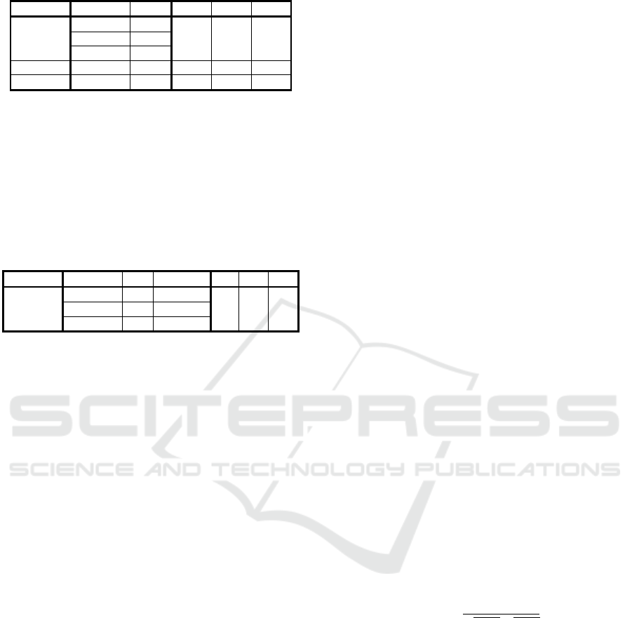
Table 2: Frequency Counting for Device States.

interval_id

time_stamp

state

s257

s258

s262

interval 1

'257'

'258'

interval 2

'262'

interval 3

'262'

In more complex cases, it is possible to specify

another column the values of which will be

aggregated for each category using a custom function

instead of simply counting the occurrence number.

For example (Table 3), we might want to find the

average temperature (column temp) for each

individual category rather than for the whole interval

(shown in Table 1).

Table 3: Aggregation for categories.

interval_id

time_stamp

state

temp

t257

t258

t262

interval 1

'257'

15.0

17.5

30.0

'257'

20.0

'258'

30.0

For proper analysis, features should be

normalized. It is especially important for imbalanced

features like event frequencies. This is due to the fact

that different categorical values have different

frequencies overall. For example, certain state

changes will be common and certain other state

changes will be rare. The absolute counts then cannot

be compared because the frequency of 10 for a

common event is very different than the frequency of

10 for an uncommon event. To normalize the

frequency data, we divide the frequency values for

each row by the total frequency of the column. Such

normalization is common also in modeling using the

bag-of-words approach where it is called TF-IDF

(Manning et al., 2008).

4 DATA ANALYSIS

4.1 Multidimensional Scaling

Rows of the table with aggregated and normalized

features can be formally treated as points in the

multidimensional space where dimensions are

columns. The task is then to find unusual points

which differ significantly from most of the other

points. We evaluated many machine learning

algorithms for identifying anomalies in such data sets

and found that Multidimensional Scaling (MDS)

(Borg & Groenen, 2005) is one of the most effective,

simple to tune, easy to understand, and visualize.

Multidimensional scaling (MDS) is one of several

multivariate techniques which aims to place objects

in N-dimensional space by preserving the between

object distances as well as possible. In other words,

MDS finds a low-dimensional (  ) representation

of the data in which the distances in the original high-

dimensional space are well respected. In our

algorithm, we have used a 2-dimensional

representation.

Multidimensional scaling identifies the new

representation by minimizing the quantity called

STRESS or SSTRESS (Kruskal, 1964):

   













 













   















 

















is the dissimilarity between i-th and j-th data

points and 



is the Euclidean distance between the

i-th and j-th data points in the new low-dimensional

representation. The parameters which minimize this

are estimated using the SMACOF (de Leeuw, 1988)

algorithm. The algorithm requires 





calculations and 



 memory. We have used the

MDS function in the scikit-learn library for

machine learning algorithms in Python.

Dissimilarity measure is an essential parameter of

MDS. Common dissimilarity measures are

Euclidean, Hamming, cosine, etc. We have used the

cosine distance as the measure of dissimilarity for our

data (this measure is also used in classifying

documents using the bag-of-words approach). The

cosine distance is defined as 1-cosine similarity

(Singhal, 2001) where cosine similarity is the cosine

of the angle between two vectors represented by data

points a and b with components 



and 











  

































Cosine distance is bounded in [0, 1] and is efficient to

evaluate as only non-zero components need to be

evaluated.

When analyzing data from robotic lawn mowers,

we used their log events to get the current state and

error status codes. Since these are categorical

features, they were transformed to normalized

frequencies as described in Section 3.3. The result

table had many columns with frequencies of specific

status codes for the chosen interval length. The goal

was to identify anomalous behavior by analyzing

these frequencies using MDS algorithm. Our

hypothesis is that anomalous devices will log events

IoTBDS 2018 - 3rd International Conference on Internet of Things, Big Data and Security

with uncommon frequencies, i.e. high-frequency for

low-frequency events or very low-frequency for

high-frequency events. It also occurred that

anomalous lawn mowers had an uncommon

combination of events, i.e. events occurring together

which usually are not.

The task of MDS is to reduce all the frequency

columns to only a few dimensions. In our case, we

chose to reduce to 2 dimensions which is easier to

visualize and interpret. MDS generates two output

dimensions, x and y, and each device is then

represented as a point in a two-dimensional space.

The anomaly score is then computed as the distance

from the origin:







 



The more a point is further away from the origin, the

more anomalous behavior it shows.

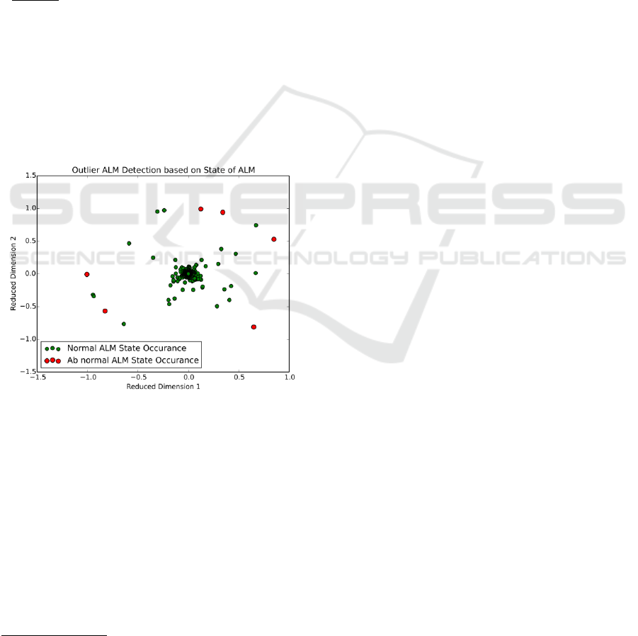
Analysis results of the MDS algorithm are

visualized as a scatterplot where anomalous devices

are highlighted and are shown as outliers (Fig. 3). The

user can hover over the points and see the detailed

information like device id and time this anomaly was

detected.

Figure 3: Scatterplot with anomalies.

4.2 Elliptic Envelope and One-Class

SVM

Although MDS showed quite good results, it cannot

be always used for two reasons:

 MDS is a computationally difficult algorithm

because it has to build an 



matrix of

distances. Therefore, it can be applied to only

relatively small data sets.

 MDS does not train a model but rather finds

anomalies by processing the whole data set.

https://bosch-iot-suite.com/

Hence, it is necessary to process the complete

history for every update, for example, when

new events have been received.

In general, it desirable to have many possible

algorithms in order to be able to compare their results.

Therefore, we also added other algorithms to our

system. The first approach is based on fitting an

ellipse to the data by assuming that the inlier data are

Gaussian distributed. This ellipse essentially defines

the “shape” of the data.

We also evaluated One-Class SVM algorithm

(Schölkopf et al., 1999; Smola & Schölkopf, 2004).

Strictly speaking, it is a novelty detection algorithm

because it assumes that the training data set is not

polluted by outliers or anomalies. Yet, it is possible

to specify a contamination parameter which

represents the fraction of outliers in the training set.

In contrast to the conventional SVM algorithm, it

learns a single class of normally behaving devices. Its

advantage is that it works without any assumptions

about the data distribution (as opposed to elliptic

envelope which learns an ellipse) and can learn

complex “shapes” of data in a high-dimensional

space. This analysis is similar to the approach

described in Khreich et al., 2017.

The model is then applied to the test data set by

returning the decision function for each event. Its

values are then scaled to the interval [0,1], stored as a

new column in the data frame and used as anomaly

score (for example, for visualization). High values of

this score close to 1 represent anomalies while points

close to the center of the distribution are treated and

having low anomaly score are treated as normal

behavior.

The results of analysis are visualized as a line plot

where the horizontal axis corresponds to time and the

vertical axis plots the anomaly score between 0 and 1

(Fig. 4).

5 IMPLEMENTATION

This approach was implemented as a cloud service in

the Bosch IoT Cloud (BIC) being also a part of the

Bosch IoT Suite

which is a cloud-enabled software

package for developing applications in the IoT. By

implementing the anomaly detection service (ADS)

as a cloud service, we get several advantages like high

scalability and better interoperability which decrease

complexity, improve time-to-market for new IoT

solutions and, for that reason, also reduce the total

cost of ownership.

Detecting Anomalies in Device Event Data in the IoT

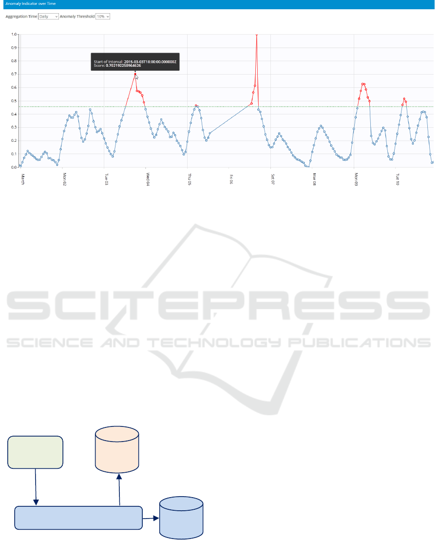
Figure 4: Time plot with anomaly score for one device.

ADS consists of the following main components

(Fig. 5):

 Cloud service (Java) exposes all functionalities

of ADS via REST API which can be used by

other services or applications. It stores all

assets in an instance of MongoDB database and

uses Splunk (Zadrozny & Kodali, 2013) for

logging.

 Executor (Java) is responsible for executing

analysis jobs initiated via REST API. It uses the

RabbitMQ message bus to receive job requests

and creates a new process for each job which

executes a Python workflow.

 Analysis workflow engine (Python) is started

by the Executor. It reads data from the specified

data source and writes the results of the

analysis into the output database.

Figure 5: Architecture of the anomaly detection service.

ADS also provides a front-end which is

implemented using AngularJS and runs in the

browser by relying on the service REST API. The

front-end has the following main functions:

 Authoring analytic workflows by creating,

editing or deleting them using a wizard instead

of writing such workflows in JSON format.

 Execute analysis jobs and tracking their

progress and status.

 Visualizing analysis results (like screenshots in

Fig. 3 and Fig. 4) or downloading them.

An analysis workflow for anomaly detection

consists of 5 steps which correspond to 5 nodes in the

Python analysis engine: read data (from a file or

database), generate new features without changing

the number of rows (as described in Section 2), define

new aggregated features by grouping rows into

intervals and then applying several aggregate

functions (as described in Section 3), choose a data

analysis algorithm (as described in Section 4), and

finally write the result with anomaly score to an

output file or database.

Fig. 6 is an example of how data aggregation step

in the analysis workflow can be defined using the

wizard. First, it is necessary to choose an aggregation

interval. In this example, it is 1 hour which means that

the behavior of devices will be analyzed on hourly

basis. In other words, any behavioral pattern or

characteristic is defined by all events from one device

for one hour. Then it is necessary to define one or

more features where each feature will analyze all

events for one hour and one device by returning one

value treated as a behavioral characteristic for this

hour. In this example, 2 features are defined. The first

feature returns mean value of the area already mowed

for all events received for one hour. The second

feature will generate as many columns as there are

state codes and for each of them it will compute their

count for this hour (Section 3.3). In order to use a

Anomaly Detection Service (ADS)

Analysis

models

Application

or Service

Event

Data

Configure models

trigger analysis

Read data

write results

REST

IoTBDS 2018 - 3rd International Conference on Internet of Things, Big Data and Security

Figure 6: Wizard page for defining aggregated features.

user-defined aggregate function, its name has to be

written in the feature definition and the function

source code has to be uploaded on the page with basic

information.

When an analysis workflow is started, then it is

scheduled for execution by waiting in the queue of

other jobs. A free Job Executor will retrieve the next

job and spawn a new OS process. This process will

get the workflow description in JSON format as a

parameter and execute all its nodes starting from data

input and ending with data output.

6 CONCLUSIONS

In this paper, we described a system for detecting

anomalies in device data with no or little numeric

characteristics. A preconfigured analysis workflow

consists of the nodes for feature generation, feature

aggregation, and data analysis. This approach was

implemented as a cloud service where it can be easily

provisioned and configured for processing specific

data sets. This approach provides the following main

benefits:

 Creating an analysis workflow for specific use

cases takes much less time in comparison to

using a general-purpose data mining tool

because we provide pre-configured analysis

templates for specific problems. In particular,

our analysis template for anomaly detection is

designed for analyzing asynchronous events

coming from a fleet of devices having multiple

sensors sending semi-structured data.

 It is easy to encode domain-knowledge into the

analysis workflow so that the necessary data

transformations and feature engineering tasks

are made an integral part of the whole analysis.

In the future, we are going to extend this project

in the following directions:

 [Enhancing analysis methods] We will develop

new approaches to anomaly detection. In our

current setup, anomalies may not be detected if

an interesting sequence of events happens

because their overall counts may not be

interesting. Therefore, we will work on using

sequence mining (Chandola et al., 2012)

algorithms to detect anomalies by finding

interesting or unusual sequences of events.

Various such techniques exist including

window-based techniques where sequences are

matched in a given window and Markovian

techniques where a Markov model of state

transition is developed and the probability of a

sequence is calculated. Different such

techniques will be experimented with.

 [Apply the same approach to other tasks] We

are going to generalize the analysis patterns

used in this project by developing similar

services for other problems like predictive

maintenance or data validation. The main idea

of such services will be the same: it is based on

a predefined analysis workflow which is easy

to be configured and used in the cloud.

Detecting Anomalies in Device Event Data in the IoT

 [Performance and scalability] From the

implementation point of view, our goal is to

make execution in the cloud more performant

and to better use the scalability features of the

cloud. These features are especially important

in the case of large-scale analysis (during

training phase) as well as for serving many

users or other applications. In particular, we

will study how existing relevant technologies

like Mesos (Hindman et al., 2011) or

Kubernetes can be used for that purpose.

REFERENCES

Abadi, D.J., 2007. Column stores for wide and sparse data.

In Proceedings of the Conference on Innovative Data

Systems Research (CIDR), 292–297.

Ahmed, M., Mahmood, A.N., Hu, J., 2016. A survey of

network anomaly detection techniques. Journal of

Network and Computer Applications 60, 19–31.

Berthold, M.R., Cebron, N., Dill, F., Gabriel, T., Koetter,

T., Meinl, T., Ohl, P., Sieb, C., Thiel, K., Wiswedel, B.,

2007. Knime: The Konstanz Information Miner.

Proceedings Studies in Classification, Data Analysis,

and Knowledge Organization (GfKL), Freiburg,

Germany, Springer-Verlag.

Borg, I., Groenen, P.J., 2005. Modern Multidimensional

Scaling: Theory and Applications. Springer, New York,

NY, USA.

Box, G.E.P., Jenkins, G.M., 1976. Time Series Analysis:

Forecasting and Control, Rev. Edition, San Francisco:

Holden-Day.

Chandola, V., Banerjee, A., Kumar, V., 2009. Anomaly

Detection: A Survey. ACM Computing Surveys 41(3).

Chandola, V, Banerjee, A., Kumar, V., 2012. Anomaly

Detection for Discrete Sequences: A Survey, IEEE

Transactions on Knowledge and Data Engineering,

24(5).

Copeland, G.P., Khoshafian, S.N., 1985. A decomposition

storage model. In SIGMOD 1985, 268–279.

de Leeuw, J., 1988. Convergence of the majorization

methods for multidimensional scaling. Journal of

Classification, 5(2):163–180.

Dean, J, Ghemawat, S., 2004. MapReduce: Simplified data

processing on large clusters. In Sixth Symposium on

Operating System Design and Implementation

(OSDI'04), 137–150.

Guyon, I., Gunn, S., Nikravesh, M., Zadeh, L.A., 2006.

Feature Extraction: Foundations and Applications.

Springer, New York, NY, USA.

Kandel, S. et al., 2011. Research Directions in Data

Wrangling: Vizualizations and transformations for

usable and credible data. Information Visualization,

10(4), 271–288.

Khreich, W., Khosravifar, B., Hamou-Lhadj, A., Talhi, C.,

2017. An anomaly detection system based on variable

N-gram features and one-class SVM. Information and

Software Technology 91, 186–197.

Kruskal, J.B., 1964. Multidimensional scaling by

optimizing goodness of fit to a nonmetric hypothesis.

Psychometrika, 29(1):1–27.

Manning, C.D, Raghavan, P, Schutze, H., 2008. Scoring,

term weighting, and the vector space model.

Introduction to Information Retrieval. p. 100.

McKinney, W., 2010. Data Structures for Statistical

Computing in Python. In Proceedings of the 9th Python

in Science Conference (SciPy 2010), 51–56.

McKinney, W., 2011. pandas: a Foundational Python

Library for Data Analysis and Statistics. In Proc.

PyHPC 2011.

Hindman, B., Konwinski, A., Zaharia, M., Ghodsi, A.,

Joseph, A.D., Katz, R., Shenker, S., Stoica, I., 2011.

Mesos: A Platform for Fine-Grained Resource Sharing

in the Data Center. Proc. 8th USENIX conference on

Networked systems design and implementation (NSDI

2011), 295–308.

Saia, R., Carta, S., 2017. A Frequency-domain-based

Pattern Mining for Credit Card Fraud Detection, In

Proc. 2nd International Conference on Internet of

Things, Big Data and Security (IoTBDS 2017), 386–

391.

Savinov, A., 2014. ConceptMix: Self-Service Analytical

Data Integration Based on the Concept-Oriented

Model, Proc. 3rd International Conference on Data

Technologies and Applications (DATA 2014), 78–84.

Savinov, A., 2016. DataCommandr: Column-Oriented Data

Integration, Transformation and Analysis.

International Conference on Internet of Things and Big

Data (IoTBD 2016), 339–347.

Singhal, A., 2001. Modern Information Retrieval: A Brief

Overview. Bulletin of the IEEE Computer Society

Technical Committee on Data Engineering, 24(4): 35–

43.

Schölkopf, B., Williamson, R., Smola, A., Shawe-Taylor,

J., Platt, J., 1999. Support Vector Method for Novelty

Detection. In Proc. 12th International Conference on

Neural Information Processing Systems (NIPS 1999),

582–588.

Smola, A.J., Schölkopf, B., 2004. A Tutorial on Support

Vector Regression. Statistics and Computing archive,

14(3): 199–222.

Zadrozny, P., Kodali, R., 2013. Big Data Analytics Using

Splunk: Deriving Operational Intelligence from Social

Media, Machine Data, Existing Data Warehouses, and

Other Real-Time Streaming Sources. Apress, Berkely.

Zaharia, M., Chowdhury, M., Das, T. et al., 2012. Resilient

distributed datasets: a fault-tolerant abstraction for in-

memory cluster computing. In Proc. 9th USENIX

conference on Networked Systems Design and

Implementation (NSDI'12).

IoTBDS 2018 - 3rd International Conference on Internet of Things, Big Data and Security