Characterization of High Speed Optical Detectors for Purpose of

OM4 Fibre Qualification: Selective Mode Detection

F. J. Achten

and D. Molin

Prysmian Group, Zwaanstraat 1, 5651CA Eindhoven, Netherlands

Prysmian Group, Parc des Industries Artois Flandres, 62092 Haisnes Cedex, France

Keywords: High Speed Optical Fibre, High Speed Detector, Optical Fibre Qualification.

Abstract: The most important characterization of OM4 fibre is the ‘Differential Mode Delay’ (DMD) measurement.

The measured DMD profile is some kind of ‘roadmap’ of the OM4 fibre; it contains all relevant data from

which the main optical parameters are computed (for instance ‘Effective Modal Bandwidth’). Most

requirements for the measurement equipment are well defined within standardization documents. However

the requirements for the detector are still under discussion. This paper shows the state of the art of

commercially available detectors (high speed optical electrical converters, fibre coupled) from different

manufacturers. A method to characterize these detectors is suggested, and it shows the ‘ideal’ detector is not

yet commercially available.

1 INTRODUCTION

In today’s world the need for high speed data

transmission is growing. In high performance data

centers multimode fibres are commonly used. Today

the operational wavelength is 850 nm, but ‘wide

band multimode fibres’, covering the range 850 nm

to 950 nm (likely to be OM5) are being developed

and tested in systems (CommScope, 2015, Molin

2014). Some publications exist to discuss the

specifications that wide band fibre should reach 950

nm (Pimpinella, 2014, Bigot, 2015)). These fibres

are qualified by a tightly standardized measurement

method called ‘Differential Mode Delay’ (DMD)

(Oh, 2012, TIA, 2003). The main parameter

considered is the ‘Effective Modal Bandwidth’

(EMB). The EMB is computed from the ‘un-

normalized DMD profile’ (TIA, 2003, IEC, 2017).

The specification for the EMB value becomes more

relaxed when the wavelength increases from 850 to

950 nm. This is caused by the fact that the ‘penalty’

caused by Chromatic Dispersion goes down. At 850

nm the EMB specification is 4700 MHz.km, at 950

nm EMB is specified at 2450 MHz.km (note: precise

value are still under discussion at IEC and TIA).

When the fibre is optimized at 850 nm, the EMB

will be much higher than the specified value.

However, when the range 850 nm to 950 nm is

considered, the EMB values at 850 nm and 950 nm

will be closer to the specified values. This means the

precision of the DMD measurement method

becomes more relevant. On the launching side (side

of the fibre where the laser pulses are launched into),

the laser pulse characteristics and the exact position

and size of the launch spot are very relevant. On the

detector side, two properties are relevant. First of all

the detector must be sufficiently fast to detect small

changes of the laser pulse shape after travelling

through the fibre under test. If fibres are measured

close to the fibre length used in systems, the laser

pulse must be very narrow in time domain (and also

in wavelength domain). A typical value for the Full

Width Quarter Max (FWQM) of the laser pulse is 10

ps. A typical value for the detector bandwidth to

proper detect this pulse is 25 GHz. The FWQM of

the pulse detected by such a detector will be typical

35 ps (referred to as ∆T

REF

Secondly, the detector must detect all the modes

guided by the fibre under test. The detector response

should be close related to the actual spatial and

angular power distribution leaving the fibre under

test. High speed detectors often tend to have a

sensitive area smaller than the field leaving the fibre

under test. The speed of the detector drastically

reduces when the diameter of the sensitive area gets

larger (Hui, 2012). To catch all the light that leaves

the fibre under test, the internal fibre pigtail of the

Achten, F. and Molin, D.

Characterization of High Speed Optical Detectors for Purpose of OM4 Fibre Qualiﬁcation: Selective Mode Detection.

DOI: 10.5220/0006541201410147

In Proceedings of the 6th International Conference on Photonics, Optics and Laser Technology (PHOTOPTICS 2018), pages 141-147

ISBN: 978-989-758-286-8

141

detector may consist of a tapered or lensed core. The

consequence of such a structure is some light will

leave the internal fibre pigtail from the side, and so it

will not reach the sensitive area of the detector. This

causes ‘selective mode detection’. Sometimes the

internal fibre pigtail is bended to fit the small

housing. This will introduce macrobend losses. As

far as we know, no commercial available detector

exists that uses a ‘bend insensitive’ fibre design as

the internal fibre pigtail. Another cause of selective

mode detection may be imperfections of the

sensitive area. If the detector suffers from selective

mode detection, the measured DMD profile of the

OM4 fibre under test is not theoretically correct, and

as a consequence the computed EMB value isn’t

correct either.

This paper describes a method to characterise a

detector, so it can be used to qualify OM4 fibre. The

method is tested on five different detectors from

different manufacturers. These detectors are all

specified for multimode fibre, with a very high

optical bandwidth of at least 10 GHz. A very high

bandwidth is mandatory to qualify short length of

OM4 fibre, for instance close to the maximum

system length of 400 m. All detectors are fibre

pigtailed with a 50 or 62.5 µm core Graded Index

fibre. Also a low bandwidth detector is used as a

reference. This detector cannot detect the individual

pulses (too slow), but can measure the power

distribution on a near DC level. Two of the used

detectors were developed for 850 nm pulse

measurement (so are not suited to qualify wide band

multimode fibres up to 950 nm). For now the

detectors are investigated at 850 nm, but the same

method (for the 950 nm sensitive detectors) can be

used for other wavelengths in the range 850 - 950 nm.

2 CHARACTERIZATION

METHOD

To characterize a detector, a special designed optical

fibre is used. Referred to as ‘mode separating fibre’.

Regular multimode fibres are designed with an

‘Alpha Profile’ refractive index core (Oh, 2012). If

the Alpha value (α) is optimized for a particular

wavelength (OM4: 850 nm), and the refractive index

profile is very accurate, the EMB reaches very high

values at that particular wavelength. This means all

launched modes reach the detector at the same time

after travelling through the fibre. The pulses are

shaped exactly equal as launched into the fibre

(assuming a short fibre length of max 1 km, so

Chromatic Dispersion effects can be neglected). A

typical value for α is 2.0. The special designed

optical fibre (‘mode separating fibre’) has an α of

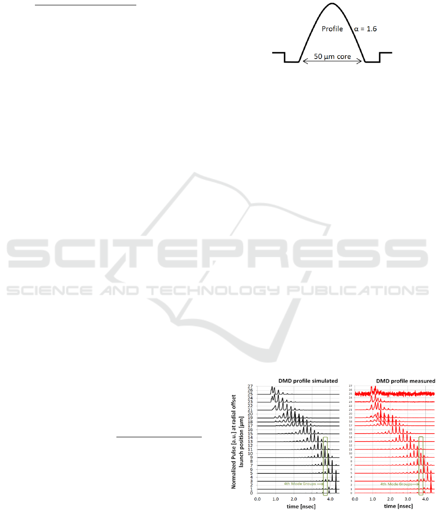
1.6. The profile is shown in Figure 1.

Figure 1: refractive index profile of the special designed

fibre (’mode separating fibre’).

Because of the low α, the mode groups experience

different times of flight through the fibre. This can

be clearly seen on the resulting (normalized)

measured DMD profile of Figure 2b (used is a

Titanium Sapphire Mode Locked laser, 10 ps pulses,

850 nm). Figure 2a shows a simulated DMD profile

on an ‘ideal’ α = 1.6 fibre. The simulation model is

described in (Gholami, 2011). The method (and

equipment requirements) to get a fibre DMD profile

is described in detail in TIA and IEC documents

(TIA, 2003, IEC, 2017). The 18 mode groups reach

the fibre end at clear different moments in time. So

one can derive the positions in time of the mode

groups leaving the fibre, and the power of the pulses

present within each mode group launched at

different radial offset positions. If the α = 1.6 fibre is

‘perfect’ (equal to the input to the simulation

model), the difference between the detected DMD

profile and simulated DMD profile is a measure for

detector performance. The closer both DMD

profiles, the better detector performance (it then

detects all mode groups leaving the α = 1.6 fibre).

The used length of the α = 1.6 fibre (mode

separating fibre) is 550 m.

a b

Figure 2: simulated and measured DMD profile after 550

m of the ’α = 1.6 fibre’ (mode separating fibre). 18 Mode

Groups are visible and clearly separated in time.

PHOTOPTICS 2018 - 6th International Conference on Photonics, Optics and Laser Technology

142

3 MODE SEPARATING FIBRE

In Graded Index (GI) multimode fibres, the modes

are sorted into mode groups. Modes of the same

mode group exhibit nearly the same group index and

the group index difference with its neighbour. Thus

the time of flight differences are nearly the same for

all mode groups. This difference of time of flight

between consecutive mode groups is at first order a

function of the alpha value (α), the numerical

aperture (NA) or Delta (Oh, 2012), the core diameter

and the wavelength of operation (λ). And at second

order a function of the dopant content (full

Germanium, full fluorine or a Germanium &

Fluorine co-doping).

For the mode separating fibre, the α value is

adapted so that the mode groups experience a clear

different time of flight when travelling through the

fibre. Visible by performing a DMD measurements

at a specific minimal fibre length. This condition

can be expressed as follows:

Δ𝜏

∙ 𝐿

ΔT

𝑅𝐸𝐹

> 𝑋

Where Δτ is the time delay difference between

consecutive mode groups in ps/m, L is the minimum

fibre length to use in the DMD measurements in m,

ΔT

REF

is the Full Width Quarter Max (FWQM) of

the ‘reference’ pulse used in the DMD measurement

in ps (the detected pulse launched to the fibre), and

X is a ‘threshold’ that is larger than 4.

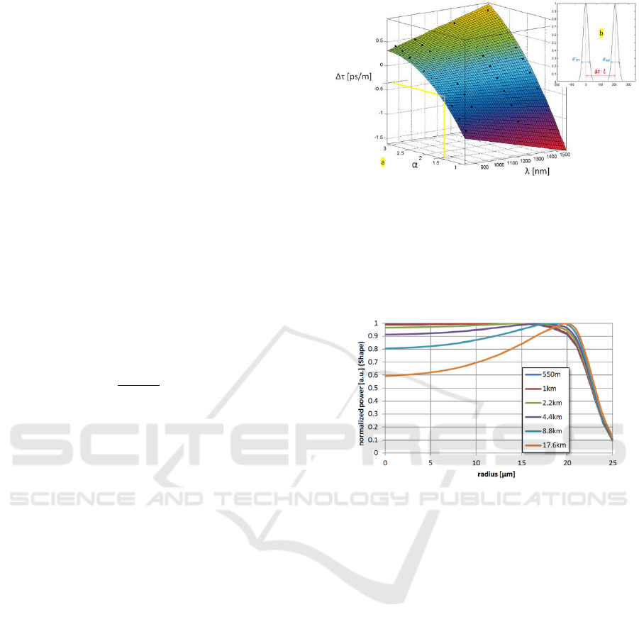
For a 50 µm core GI multimode fibre with an

NA = 0.200, one can approximate Δτ as follows:

Δ𝜏

(

𝜆, 𝛼

)

= 𝑃

+ 𝑃

∙ 𝜆 + 𝑃

∙ 𝛼 + 𝑃

∙ 𝜆 ∙ 𝛼

+ 𝑃

∙ 𝛼

The constants P

are computed using a simulation

model (Gholami, 2011), the result is shown in

Figure 3a. Figure 3b shows the pulses leaving the

fibre, referring also to Figure 1. When α = 1.6 → Δτ

= 0.36 ps/m, so the delay between 2 mode groups

after 550 m fibre is 200 ps.

The total power of all mode groups leaving the

fibre depends on the launch radial offset. While

approaching the edge (25 μm) of the core, the power

will go down (some pulse energy is launched in the

cladding, and power is lost because of core-cladding

interface artefacts and slight fibre bending). The

distribution of the power over the core radius

depends also on the length of the fibre.

Figure 3: (a) 3-D plot showing which α suits best for the

mode separating fibre (α = 1.6), used at a specific

wavelength, to reach a clear separation of the mode groups

after travelling through the fibre (b).

Figure 4 shows the theoretical power distribution

over a Graded Index 50 μm core fibre. From now on

referred to as ‘Shape’.

Figure 4: Theoretical power distribution (’Shape’) over a

Graded Index 50 μm core fibre. The distribution changes

with fibre length.

Note: the shape of the trace shows a ‘dip’ in the

centre as the fibre gets longer. This is because of the

higher Ge content near the centre of the core, so

attenuation increases faster with length for light

travelling through the centre region of the core.

The mode separating fibre is a useful tool to

characterize a detector on selective mode detection,

to verify whether the detector is suited to qualify

OM4 fibre; detect DMD profiles with maximum

accuracy.

4 THE DETECTORS

According to the DMD measurement standard (TIA,

2003, IEC, 2017), the detected launch pulse should

have a FWQM below a certain value. This value

(∆T

pulse

) depends a.o. on the spectral width of the

laser (δλ), the chromatic dispersion of the fibre

(D(λ)) and the length of the fibre. The lowest DMD

Characterization of High Speed Optical Detectors for Purpose of OM4 Fibre Qualiﬁcation: Selective Mode Detection

143

values to be measured with sufficient accuracy

depends on ∆T

pulse

. For OM4 fibre the specification

is 0.10 ps/m. Figure 5 shows the relation between

fibre length and the minimum required value for

∆T

pulse

(for the used laser and fibre: δλ = 0.1 nm,

D(λ)= 95 ps/nm.km). The experiments are done on

the mode separating fibre with a length of 550 m.

Figure 5: laser pulse and detector requirements to qualify

OM4 fibre at different lengths.

A total of five commercially available detectors is

studied. It is not the intention to review these

detectors, and promote the best performing detector.

The intention is to review commercial availability of

very high speed multimode detectors that are

mandatory for OM4 fibre qualifications when short

fibre length are measured. For instance 400 meter,

the maximum system length. The five detectors are

all commercially available (high speed optical

electrical converters, fibre coupled, some less easy

to find), and will be left anonymous. The exact

internal structure of some of these detectors is

unknown.

Detector #1 is an integrated optical-electrical

module (responsivity in A/W is not specified). The

detectors #2 and #5 use an internal tapered pigtail;

the sensitive detection area is near 30 µm diameter.

Detector #3 is special because it is very fast (45

GHz), despite using a ‘direct’ coupling of the 50 µm

internal pigtail to the sensitive detection area

(without internal fibre lensing or tapering). The

relatively large area must be thin to reach the high

detection speed, and as a consequence the

responsivity is very low (Hui, 2012).

For instance, from Figure 5, it shows detector #1

is too slow (10 GHz), case an OM4 fibre is

measured at maximum system length (400 m), the

specified detector bandwidth should then at least be

20-25 GHz. Only four of such detectors (multimode,

≥ 20 GHz) are commercially available to date and to

our knowledge.

5 MEASUREMENT RESULTS

5.1 Reference

First objective is to verify the theoretical Shape

using 550 m of the α = 1.6 test fibre. The only way

to verify this is using an optical detector with an

homogeneous sensitive area significantly larger than

the modes field diameter of the light leaving the α =

1.6 fibre. The output of the fibre must be radiated

directly on the sensitive area of the detector, no

optics (or fibre) in between. This measurement is

done by performing a ‘DMD scan’ in 4 directions

(4-Quadrant scan: 4Q). The way to do this is well

described in the standardization documents (TIA,

2003, IEC, 2017). The laser source we use is a 10 ps

Titanium Sapphire Picosecond laser. The 4Q scan

enables accurate alignment of the fibre, so the

launch at 0 µm radial position indeed is at the optical

centre of the fibre. After the DMD scan, the 4

quadrants are combined, for instance by folding the

pulses at each launch radius. The pulses leaving the

fibre normally go to the high speed detectors under

test, connected to a sampling module and signal

analyser. However the large area detector is too slow

to follow the fast Ti:Sapp laser pulses, so the

incoming beam is modulated with a chopper at 160

Hz, connected to a Lock In Amplifier. At each radial

launch position the signal is measured. Finally the 4

quadrants are averaged, resulting in the results

shown in Figure 6.

Figure 6: theoretical and verified ‘DC ’power distribution

(Shape) after 550 m α = 1.6 fibre.

PHOTOPTICS 2018 - 6th International Conference on Photonics, Optics and Laser Technology

144

(a)

(b)

(c)

Figure 7: (a) reproducibility of detectors #3 and #4.

(b) Shape of all five detectors.

At the outer launch positions (23 & 25 µm from the

centre), the experiment shows higher power, we

believe this difference is caused by inaccuracies in

the fibre index profile close to the cladding

(scattering, leaky modes). Up to 23 µm theory and

experiment are almost in accordance.

5.2 Detectors under Test

The coupling of laser pulses into the α = 1.6 fibre is

realized by a direct coupling of a HP780 launch fibre

(single mode at 850 nm, launch spot diameter 5 μm)

to the α = 1.6 fibre. For both fibres, the cleave quality

is checked by an interferometric technique, and is far

below an angle of 1 degree (to avoid angular coupling

to the α = 1.6 fibre). The 4Q DMD scan (including

alignment, 850 nm) is executed five times per detector

to visualize the reproducibility of the measurement.

For detectors #3 and #4 the five power distributions

(‘Shapes’) are shown in Figure 7a. The responsivity

of detector #3 is very low, causing this detector to

have the poorest reproducibility. Figure 7b shows the

power traces (Shape) of all five detectors.

It is clear that none of these detectors reach the

theoretical Shape. Since the exact internal structure of

the detectors in unknown, it is hard to explain the

observed differences.

5.3 Discussion

The internal fibre pigtails of detectors #2 and #5 are

‘tapered’. So the pigtail output field to the detector

sensitive area is reduced to a smaller area (from 62.5

to 30 μm diameter). In some way modes are lost, and

do not reach the sensitive area (or reach the area, but

do not generate current). It makes sense the lost

modes are the modes that travel closest to the

cladding. The Shape for both detectors is nearly

equal, detector 2 is slightly closer to the theoretical

Shape (detector 2 has a slightly lower bandwidth, so

maybe the sensitive area is just a little larger).

Detector #1 shows a Shape equivalent to #2 and

#5, which might mean it is also equipped with an

internal tapered (or lensed) fibre pigtail.

Detector #3 is the oddball of the selection. It has

an internal 50 µm pigtail that is not tapered or lensed,

and -as a consequence-, uses a larger and thinner

sensitive area. So it causes a significantly lower

responsivity (Hui, 2012). Still, the Shape does not

reach theory. For the outer part (narrow shape) two

explanations might be considered: bend losses of the

internal pigtail (50 µm shows more bend loss

compared to 62.5 µm), as the pigtail is bended over

few cm inside the detector housing. We also noticed a

poor coupling of the pigtail to the sensitive area

(slight mismatch). An interesting solution might be to

use ‘bend-insensitive’ 50 µm fibre as the internal

pigtail. The ‘dip’ in the middle is more difficult to

explain. Possibly the homogeneity of the sensitive

detector area is poor because it needs to be thin to

reach the high speed (45 GHz).

Characterization of High Speed Optical Detectors for Purpose of OM4 Fibre Qualiﬁcation: Selective Mode Detection

145

(a)

(b)

(c)

(d)

Figure 8: Detected mode group powers of the #3 detectors

considered at launch radii of 0 μm (centre), 9 μm (most

mode groups detected), 18 μm (relevant for ‘inner’ DMD),

and 23 µm (‘outer’ DMD).

Finally detector #4. The Shape is ‘roundish’. The

size of this detector is very small, and it is

completely sealed. The internal structure is

unknown. This detector proves to be the least suited

to qualify OM4 fibre; it shows the narrowest shape

of all five detectors.

5.4 A Closer Look

The previous results will show as well by using a

regular OM4 fibre rather than the α = 1.6 fibre; the

differences in Shape are almost equivalent. Using

the α = 1.6 fibre however generates the ability to

verify the detector response not only per launch

offset radius, but also per mode group. To simplify

analysis, we consider detectors #2 (widest Shape),

#3 (centre dip) and #4 (narrowest Shape).

In Figure 8 the detected powers per mode group

at 4 launch offset radii are plotted together with

theoretical values derived from the simulated DMD

profiles (detector #2 shown in Figure 2a).

To scale the power levels equal, it is assumed at

9 μm radial offset, all mode groups are detected.

From Figure 2 it shows the agreement between the

simulated and measured DMD profile (detector #2)

is fair, however when approaching the cladding, the

differences increase. This is probably caused by

core-cladding interface artefacts of the α = 1.6 fibre.

Further, to optimize the model, one must know the

exact Alpha value, core-size and Delta (Oh, 2012),

and these must be very constant over full length (550

m) of the α = 1.6 fibre (here’s another challenge).

From Figure 8a, theory, ‘odd’ mode groups are

symmetric whereas ‘even’ mode groups are anti-

symmetric (Gholami, 2011). So no power at fibre

output by the even mode groups. This is well

confirmed by the experimental data.

Detector #3 fails to detect full power of the first

mode group, while the third and fifth mode group

approach theory. Probably caused by an artefact in

the centre of the detector sensitive area, which is a

reason to reject detector #3 for OM4 fibre

qualification.

Figure 8b and 8c show a typical but unexpected

result. The measured mode group power

distributions of the three detectors shift to higher

order modes compared to theory. One might expect

the opposite as higher mode groups are more

sensitive to selective mode detection. We expect this

is caused by local imperfections of the index profile

of the mode separating fibre (α = 1.6 fibre, figure 1).

This observation needs further research.

Figure 8d, when launching close to the cladding,

it clearly shows the loss of power for all three

PHOTOPTICS 2018 - 6th International Conference on Photonics, Optics and Laser Technology

146

detectors compared to theory. Main cause of the

narrow experimental Shapes shown in Figure 7b.

6 CONCLUSIONS

To date, to our knowledge, no commercial available

high speed detector (≥ 20 GHz) exists that can detect

all modes leaving the OM4 fibre under test.

We made a specially designed ‘mode separating

fibre’, and we used this fibre to characterize

performance of five commercially available high

speed detectors. The method clearly shows the

limitations of these detectors to qualify OM4 fibre.

Which does not mean these fibres will fail in

systems, it just shows the ideal detector for

qualifying OM4 fibre is not yet commercially

available. The next challenge is to explain the

observed mode selective detection by considering

the internal structure of these detectors in detail.

Another challenge is to bring simulated and

measured data closer by improving the quality

(accuracy of index profile and homogeneity over

length) of the mode separating fibre. From there

improvement to the detector design may lead to the

‘perfect’ detector for purpose of OM4 fibre

qualification. A first improvement to the internal

structure of the detector might be to use a ‘bend-

insensitive’ Graded Index multimode fibre to serve

as internal pigtail. This will cause less modes to

leave the pigtail from the side.

ACKNOWLEDGEMENTS

The authors would like to thank J.G.A. Achten,

retired teacher technical English, for reviewing this

paper.

REFERENCES

CommScope, 2015. Wideband Multimode Fiber - What is

it and why does it makes sense? (White paper)

http://www.commscope.com/docs/wideband_multimo

de_fiber_what_why_wp-109042.pdf

Molin D., Achten F., 2014. WideBand OM4 Multi-Mode

Fiber for Next-Generation 400Gbps Data

Communications, IWCS 2014.

Oh, K., Paek, U., 2012. Silica Optical Fiber Technology

For Devices And Components (Chapter Five), A John

Wiley & Sons, Inc, 2012.

Pimpinella, R., Kose, B., Castro, J., 2014. Wavelength

Dependence of Effective Modal Bandwidth in OM3

and OM4 Fiber and Optimizing Multimode Fiber for

Multi-Wavelength Transmission, IWCS 2014.

Bigot, M., Molin D., 2015. Wide-Band OM4 Multimode

Fibers for Future 400Gbps and 1.6Tbps WDM

Systems, IWCS 2015.

TIA, 2003. FOTP-220 - Differential Mode Delay

Measurement of Multimode Fiber in the Time Domain

– TIA-455-22-A, January 2003.

IEC, 2017. IEC 60793-1-49 ED3 - Optical fibres - Part 1-

49 (Draft): Measurement methods and test procedures

- Differential mode delay, February 2017.

Hui, R., O’Sullivan, M., 2012. Fiber Optic Measurement

Techniques (Chapter 1, pg 35). Elsevier Academic

Press, 2009.

Gholami, A., Molin, D., Sillard, P., 2011. Physical

Modeling of 10 GbE Optical Communication Systems.

Journal of Lightwave Technology, Vol. 29, No. 1,

January 2011.

Characterization of High Speed Optical Detectors for Purpose of OM4 Fibre Qualiﬁcation: Selective Mode Detection

147