CNN Patch–Based Voting for Fingerprint Liveness Detection

Amirhosein Toosi, Sandro Cumani and Andrea Bottino

Department of Control and Computer Engineering of the Politecnico di Torino, Torino, Italy

Keywords:

Fingerprint Spooﬁng, Deep Learning, Fingerprint Segmentation, Patch based Classiﬁcation.

Abstract:

Biometric identiﬁcation systems based on ﬁngerprints are vulnerable to attacks that use fake replicas of real

ﬁngerprints. One possible countermeasure to this issue consists in developing software modules capable of

telling the liveness of an input image and, thus, of discarding fakes prior to the recognition step. This pa-

per presents a ﬁngerprint liveness detection method founded on a patch–based voting approach. Fingerprint

images are ﬁrst segmented to discard background information. Then, small–sized foreground patches are

extracted and processed by a well–know Convolutional Neural Network model adapted to the problem at

hand. Finally, the patch scores are combined to draw the ﬁnal ﬁngerprint label. Experimental results on well–

established benchmarks demonstrate a promising performance of the proposed method compared with several

state-of-the-art algorithms.

1 INTRODUCTION

Nowadays, the use of ﬁngerprints as authentication

system is becoming more and more pervasive (Mal-

toni et al., 2009), as witnessed by the fact that

these sensors are starting to be deployed to un-

lock consumer devices, like notebooks and mobile

phones, and granting access to common facilities, like

schools, health clubs and hospitals. However, the use

of these devices raises several security concerns, since

they are vulnerable to more or less complicated form

of attack, which might result in granting access to

unauthorized persons.

Attacks can be both direct, operating on the sen-

sors by means of fake replica of real ﬁngerprints, and

indirect, targeting one or more of the inner modules

of the whole recognition system. Clearly, direct at-

tacks are the most easy to implement for an intruder.

Fingerprint replicas to be presented to the sensor can

be obtained by creating a mold from a latent or real

ﬁngerprint, and then ﬁlling it with materials like La-

tex, gelatin, vinyl or wood glue and so on. It has been

demonstrated that even a high quality digital image of

a ﬁngerprint is sufﬁcient (arsTECHNICA, 2013). The

literature shows the the success rate of such attacks

can be higher than 70% (Matsumoto et al., 2002),

highlighting the need for speciﬁc protection methods

capable of identifying live samples and rejecting fake

ones.

System capable of telling the liveness of a ﬁnger-

print can be broadly divided in two main categories.

On one side, we have the hardware approaches, which

tries to combine different sensors capable of detecting

the typical liveness signs of a real ﬁnger, like temper-

ature, pulse and skin resistance. However, on most

low-cost and commercial devices this is not the most

desirable solution, since it is invasive, it increases the

cost and it cannot easily tackle novel and more so-

phisticated form of attacks. On the contrary, the soft-

ware methods are cost–effective solution that rely on

adding an extra software module to the processing

chain that is capable of telling a live from a fake ﬁn-

gerprint.

Software methods can be further divided into dy-

namic, which analyzes an image stream, and static,

which process a single ﬁngerprint scan. Again, static

methods are usually preferable since they require less

data, less computational resources and can be applied

as well to sensors that cannot output an image stream.

In the literature, the problem of static software

liveness detection has been tackled in different ways.

The initial approaches were based on the observation

that the fakes are usually characterized by a lower

image quality and, thus, they were trying to analyze

some quality indexes based on a plethora of differ-

ent holistic features (Abhyankar and Schuckers, 2006;

Nikam and Agarwal, 2008; Marasco and Sansone,

2010; Galbally et al., 2012).

However, comparisons on public benchmarks

show that the discriminative power of holistic fea-

Toosi A., Cumani S. and Bottino A.

CNN Patch–Based Voting for Fingerprint Liveness Detection.

DOI: 10.5220/0006582101580165

In Proceedings of the 9th International Joint Conference on Computational Intelligence (IJCCI 2017), pages 158-165

ISBN: 978-989-758-274-5

tures is rather low, and that better performances can

be obtained by local image descriptors (Gragnaniello

et al., 2015a; Gragnaniello et al., 2015b). Initial

attempts exploited various standard descriptors like

Local Binary Pattern (LBP), Weber Local Descrip-

tor (WLD), Binary Statistical Image Features (BSIF)

and Local Phase Quantization (LPQ), Scale-Invariant

Feature Transform (SIFT), DAISY and the Scale-

Invariant Descriptor (SID). Recently, interesting re-

sults have been obtained with the introduction of

descriptors expressly designed for ﬁngerprint live-

ness detection, like the Histogram of Invariant gradi-

ents (HIG) (Gottschlich et al., 2014), the Local Con-

trast Phase Descriptor (LCPD) (Gragnaniello et al.,

2015b), and the Convolutional Comparison Pattern

(CCP) (Gottschlich, 2016).

Other approaches tried to improve the classiﬁca-

tion accuracies by combining in various ways multi-

ple handcrafted features. Examples are SVM classi-

ﬁcation of LPQ and LBP (Ghiani et al., 2012), the

integration of various image ﬁlters and statistic mea-

sures (Pereira et al., 2012), LPQ+WLD and SVM

classiﬁcation (Gragnaniello et al., 2013), various local

descriptors combined with SVM or Multi-Task Joint

Sparse Reconstruction (Toosi et al., 2015). These

works demonstrate the effectiveness of feature fusion

approaches compared to the ones based on individual

features.

The recent successes of Convolutional Neural

Networks (CNN) and Deep Learning approaches in

a number of large scale visual recognition and clas-

siﬁcation challenges (like MNIST, ImageNet, CIFAR

and so on), stimulated their introduction in the area

of ﬁngerprint liveness detection. The deep learning

approaches to liveness detection can be roughly di-

vided in two classes. The ﬁrst class includes meth-

ods that create ad–hoc models, such as (Kim et al.,

2016), which proposes a Deep Belief Network (DBN)

with multiple layers of restricted Boltzmann ma-

chine, and (Menotti et al., 2015), which presents

spoofnet, a deep CNN architecture, created by opti-

mizing both the architecture hyperparameters and the

ﬁlter weights, which was able to greatly improve the

results of other state–of–the–art approaches.

The second class includes methods based on

Transfer Learning approaches, whose rationale is to

exploit the knowledge learned while solving a prob-

lem and apply it to a similar problem in a different

context. The general approach is to adapt to the prob-

lem at hand models that have demonstrated state–of–

the–art performances in a variety of image recogni-

tion benchmarks. Examples can be found in (Menotti

et al., 2015; Nogueira et al., 2016), where several pre-

trained models, like AlexNet, VGG and CIFAR-10,

were analyzed.

The objective of our work is to further investigate

the effectiveness of CNN based Transfer Learning ap-

proaches in the context of ﬁngerprint liveness detec-

tion. In particular, we focused on AlexNet, which is a

well known model originally designed and trained to

recognize objects in natural images, showing state–

of–the–art results in the ILSVRC-2012 competition.

In contrast with previous TL approaches, after

a preliminary segmentation step aimed at discard-

ing (noisy) background information, we divide ﬁn-

gerprint images into non–overlapping patches, which

are then individually classiﬁed by the neural network.

The classiﬁcation scores computed for each patch are

then combined to obtain the ﬁnal image label.

The rationale of our approach is twofold. First,

using patches as samples rather than the full images

allow us to increase the size of the training set, thus

(hopefully) making the classiﬁer more robust and in-

creasing its generalization capabilities. Second, since

the dimension of the network input layer is neces-

sarily limited, using small sized patches allows us

to avoid resizing the samples and, thus, to retain the

original resolution and image information.

In the following section, we will detail our ap-

proach. Then, we will introduce the datasets used in

our experiments and we will thoroughly discuss the

results obtained before drawing the conclusions.

2 METHODOLOGY

As we stated in the introduction, our approach is

based on four steps:

(i) segmentation of the input test sample, in order to

divide the ﬁngerprint image into foreground, i.e.

the region of interest (ROI), and background;

(ii) extraction, from the ROI, of a set of small-sized

patches that contain foreground pixels only. The

obtained patches are normalized and fed indi-

vidually to the network;

(iii) classiﬁcation of each patch with a modiﬁed ver-

sion of the AlexNet architecture, adapted to the

problem at hand;

(iv) computation of the ﬁnal label on the base of the

patch scores.

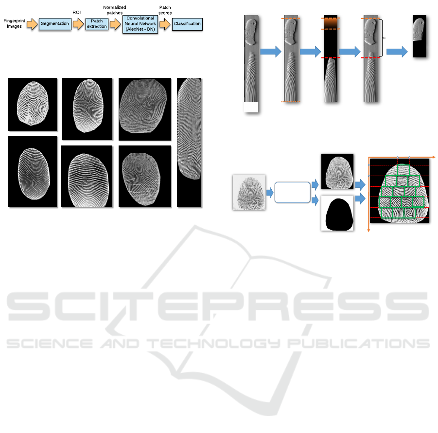
These steps are summarized in Fig. 1 and detailed

in the following subsections.

2.1 Segmentation

Fingerprint segmentation is based on the method pro-

posed in (Thai et al., 2015), which is built upon the

Segmentation

Fingerprint

Images

ROI

Patch

extraction

Normalized

patches

Convolutional

Neural Network

(AlexNet - BN)

Classification

Patch

scores

Figure 1: Outline of the proposed ﬁngerprint liveness de-

tection approach.

Figure 2: Examples of segmented ﬁngerprint images from

different sensors: (a) Sagem 2011 (b) Italdata 2011 (c)

Biometrika 2013 (d) Italdata 2013 (e) Digital 2011 (f)

Biometrika 2011 and (g) Swipe 2013.

preliminary observation that the patterns of ﬁnger-

print images have frequencies only in speciﬁc bands

of the Fourier spectrum. In order to preserve these fre-

quencies, the Fourier transform of the original image

is ﬁrst convolved with a directional Hilbert transform

of a Butterworth bandpass ﬁlter, obtaining 16 direc-

tional sub-bands. Then, soft-thresholding is applied

to remove spurious patterns. Finally, the feature im-

age is binarized and the ﬁnal segmentation is obtained

by means of morphological operators. The method is

characterized by a set of hyperparameters that are ﬁne

tuned per benchmark. This is done by optimizing the

segmentation error on a small set of manually seg-

mented images (around 30), which are taken from the

training set to include both live and fake samples cre-

ated with different spooﬁng materials. Some exam-

ples of the segmentation results can be seen in Fig. 2.

The only exception to this procedure is repre-

sented by one of the benchmarks used in our ex-

periments, the Swipe 2013 dataset (see Section 3.1),

whose images are obtained by swiping the ﬁngerprint

on a linear scanner. In some cases, these images in-

clude other ﬁnger parts beyond the pulp (the ﬁnger

extremity). When this happens, we noticed that the

segmentation algorithm might be “attracted” by these

parts discarding the pulp. Thus, for Swipe 2013 im-

ages, we adopted a slightly different procedure. First,

we removed the blank rows at the image bottom and

identiﬁed beginning and end of the impressed ﬁnger-

print by detecting large peaks of the gradient between

Incorrect

Segmented image

Original

image

Cropped

image

Remove

white space

Segmentation

(FDB Algorithm)

Compare top

ROI boundary

with starting

row of the

segmented

image

Identify

Region of

interest

boundaries

(top & bottom)

Crop and

Re-segment

(FDB Algorithm)

Figure 3: An example showing the segmentation algorithm

applied to Swipe 2013 images.

Segmentation

algorithm

(FDB)

Fingerprint

image

Segmented

image

Mask image

(ROI)

i + 64

j + 64

Figure 4: Example of the subdivision in patches of a seg-

mented ﬁngerprint for a patch size w = 64.

consecutive image lines. We then applied the segmen-

tation algorithm to the extracted region. Clearly, a

successful segmentation should start at the beginning

of this region. If, on the contrary, it starts below a

certain line (which we heuristically ﬁxed at the value

300), we take the starting line of the (incorrectly) seg-

mented area as lower boundary of the actual ﬁnger-

print region and we apply again the segmentation to

obtain the ﬁnal foreground mask (see Fig.3 for an ex-

ample).

2.2 Patch Extraction and Normalization

The segmentation mask deﬁnes the ROI where the

next computation steps are focused. This region is

divided into patches of size w × w pixels, where w is

a parameter of the method. In order to avoid any in-

ﬂuence of background pixels, we only extract those

patches whose pixels are all labeled as foreground.

The algorithm works in the following way.

We scan line by line the ROI starting from its top–

left corner and treating each (i, j) pixel as the top–left

corner of a candidate patch. If all pixels of this patch

belongs to the ROI and are labeled as foreground,

the patch is stored and the ROI scan restarts at pixel

(i + w, j). When the scan of line j is concluded, if

no patches have been found, the scan restarts at line

j + 1, otherwise at line j + w (see Fig. 4).

Finally, we normalize each patch to zero mean and

unit variance before feeding it to AlexNet.

Input

Convolution 1

Convolution 2

Convolution 3

Convolution 4

Convolution 5

Dense 1

Dense 2

Dense 3

55 x 55 x 48

27 x 27 x 128

13 x 13 x 192

13 x 13 x 128

4096 4096

Max pooling

W x W x 1

11 x 11

5 x 5

3 x 3

Batch

Normalization

Batch

Normalization

Batch

Normalization

Batch

Normalization

Batch

Normalization

Max pooling

Figure 5: AlexNet-BN Architecture.

2.3 Fine Tuning the Pre–trained

AlexNet Model

The overall AlexNet model, as used in our work,

is substantially equivalent to the one described

in (Krizhevsky et al., 2012) and summarized in Fig. 5.

In brief, the network architecture contains ﬁve

convolutional layers, interwoven with three sub sam-

pling layers, followed by three fully–connected lay-

ers. The receptive ﬁeld of each convolutional layer

is decreased from 11 in ﬁrst layer to 5 in the second

and 3 in the remaining ones. The network uses Rec-

tiﬁed Linear Unit (ReLU) as activation function, in

order to decrease the learning time and induce spar-

sity in the computed features. The size of the input

layer is w ×w × 1. In our work, we replaced the origi-

nal 1.000–unit soft–max classiﬁcation layer (designed

to predict 1.000 different classes, (Krizhevsky et al.,

2012)), with a 2–unit soft–max layer, which provides

an estimation of posterior probabilities of live and

fake classes.

As for the network weights, we started from a ver-

sion of AlexNet pre–trained on the ILSVRC–2012

dataset. This model was originally designed to rec-

ognized different categories of objects (like animals,

vehicles, buildings and so on) in natural images. This

is a domain which is substantially different from that

of our work (ﬁngerprint images), and thus the network

weights needs to be “adapted” to the actual context.

This is done by ﬁne–tuning them with a further train-

ing step that exploits the patches extracted from our

ﬁngerprint datasets. As a further detail, since we use

grayscale patches while the original AlexNet accepts

as input RGB color images, we simply picked the ﬁrst

channel of the weights of the ﬁrst convolutional lay-

ers. As a note, we also tried to transform our samples

from grayscale to color ones by simply replicating the

image plane three times, with no signiﬁcant differ-

ences. Stochastic gradient descent is used to ﬁne tune

the network weights.

Both data augmentation (see Section 2.3.1) and

dropout regularization (Srivastava et al., 2014), ap-

plied to the ﬁrst two fully connected layers with prob-

ability 0.5, have been used to soften the overﬁtting

issues. As suggested in (Simon et al., 2016), we also

used Batch Normalization (BN) to improve the net-

work performances. BN, ﬁrst proposed in (Ioffe and

Szegedy, 2015), aims at stabilizing the learning pro-

cess and decreasing the learning rates by reducing the

internal covariance shift.

2.3.1 Data Augmentation

Data Augmentation (DA) is a well–known technique

that consists in creating synthetic training samples by

applying small variations to the original data. In the

case of images, such variations are usually obtained

by applying various combination of afﬁne transforma-

tions and image cropping (Krizhevsky et al., 2012).

The advantage of DA is that it “forces” the classiﬁer

to learn small variations of the input data, thus mak-

ing it (possibly) more robust to unseen data, and it

can also act as a regularizer in preventing overﬁtting

in deep neural networks (Simard et al., 2003).

In our work, we created ﬁve different variations

of each ﬁngerprint image by (i) mirroring the image,

(ii) rotating the image of −22.5 and +22.5 degrees,

and (iii) mirroring the rotated images. Then, after ap-

plying the same transformations to the segmentation

masks, all augmented version of the input samples are

divided in patches according to the process described

in Section 2.2

As a result, the total number of training patches

after the DA step is listed, for each benchmark, in Ta-

ble 1. We underline that the augmentation process is

applied to the training set only and not to the test sam-

ples.

2.4 Patch based Classiﬁcation

The liveness of an input ﬁngerprint image is deter-

mined by combining the scores of each of the sample

patch, where as patch score we take the difference of

the two outputs of last fully connected layer (before

softmax). These scores are averaged to produce an

image score. The scores can be interpreted as log–

likelihood ratios between live and fake hypotheses,

and the image can be labeled by simply comparing the

score to a threshold τ. Theoretically, the optimal accu-

racy should obtained by setting τ = 0. In practice, we

have observed that the scores are not well calibrated,

i.e., the optimal accuracy is achieved with a differ-

ent value of τ. In order to “recalibrate” the scores,

we adopted a strategy that has been successfully em-

ployed in speaker veriﬁcation tasks (Br

ummer et al.,

2014). The method assumes that the scores for live

and fake images can be modeled by means of Gaus-

sian distributions, whose parameters can be estimated

on a validation set. Given a score s, the calibrated

score s

cal

is obtained by computing the log–likelihood

ratio

cal

= log

N (s; µ

, σ

)

N (s; µ

, σ

)

(1)

where µ

, σ

and µ

, σ

denote the mean and standard

deviation for the live and fake uncalibrated scores, re-

spectively. The sample label is then obtain by com-

paring the calibrated score s

cal

with the theoretical

threshold τ = 0.

We underline that if no patches can be extracted

from a test sample, we arbitrarily assign the fake la-

bel to the ﬁngerprint. This choice derives from the

observation that having a false fake is better than a

false live, which could result in granting unauthorized

access to the system.

3 RESULTS AND DISCUSSION

In the following, we describe the results of our exper-

iments. First, we introduce the experimental bench-

marks (Section 3.1). Then, we analyze the effect

of various parameters on the ﬁnal accuracies (Sec-

tion 3.2) and, ﬁnally, we assess our results with a

comparison with the current state–of–the–art (Sec-

tion 3.3).

3.1 LivDet Datasets

The benchmarks used in this work are those made

publicly available for the LivDet 2011 (Yambay et al.,

2012) and LivDet 2013 (Ghiani et al., 2013) compe-

titions. These datasets have been largely used in the

literature and enable a comparison with a great vari-

ety of methods and, in particular, with previous deep

learning based approaches.

Overall, the benchmarks consist in eight sets of

live and fake ﬁngerprints acquired with different de-

vices (Table 1), all of which are equipped with ﬂatbad

scanners, with the exception of Swipe, which has a

linear sensor. Its images are obtained by swiping the

ﬁngerprint and thus include a temporal dimension as

well. Each dataset is divided into separate training

and test sets, and is characterized by a different image

size and resolution, number of individuals, number of

fake and live samples and number and type of mate-

rials used for creating the spoof artifacts. Six out of

the eight fake sets were acquired using a consensual

method, where the subject actively cooperated to cre-

ate a mold of his/her ﬁnger, increasing the challenges

related to the analysis of these datasets.

According to the standard LivDet protocols, in the

following, the results are reported in terms of the Av-

erage Classiﬁcation Error (ACE), which is the av-

erage between the percentage of misclassiﬁed live

(ferrlive) and fake (ferrfake) samples, i.e. ACE =

f errlive+ f err f ake

3.2 Effect of Method Parameters

A ﬁrst set of experiments aimed at analyzing how the

various method parameters affect the recognition ac-

curacy. In particular, we investigated the contribution

of patch size, data augmentation, Batch Normaliza-

tion, and of the score calibration used in the ﬁnal clas-

siﬁcation step. A summary of these results is available

in Table 2.

The patch size controls the granularity of the

data, and we experimented with two different values,

namely 32× 32 and 64 × 64. In these experiments we

used data augmentation, batch normalization and the

calibrated scores. The results show that, in most of

the cases, using a size of 64 × 64 guarantees signiﬁ-

cant improvements of the accuracies.

On the base of the previous results, the contribu-

tion of the other parameters were evaluated with the

“optimal” patch size (i.e., 64 × 64) and by deactivat-

ing one parameter at a time. As for the data augmen-

Table 1: Characteristics of the dataset used in the experiments.

Dataset LivDet2011 LivDet2013

Scanner Biom. Digital Italdata Sagem Biom. XMatch Italdata Swipe

Image size 312x372 355x391 640x480 352x384 312x372 800x750 480x640 1500x208

Live samples 2000 2004 2000 2009 2000 2500 2000 2500

Fake samples 2000 2000 2000 2037 2000 2000 2000 2000

Total subjects 200 82 92 200 45 64 45 70

Spoof materials 5 5 5 5 5 5 5 5

Co-operative Yes Yes Yes Yes No Yes No Yes

Training slices 106,952 123,659 125,344 132,120 99,272 151,142 112,298 256,472

Table 2: Inﬂuence of method parameters on the classiﬁcation errors.

Dataset LivDet2011 LivDet2013

Parameter Biom. Digital Italdata Sagem Biom. XMatch Italdata Swipe

w = 32 7.0 3.1 8.5 5.1 0.8 12.7 0.4 7.2

w = 64 4.0 4.5 6.3 3.7 0.4 5.4 0.5 1.3

No DA (w = 64) 5.4 4.3 7.3 4.1 0.5 6.8 0.4 1.8

No BN (w = 64) 6.3 4.9 6.8 3.1 0.5 8.0 0.5 1.4

No calib. (w = 64) 4.0 5.1 6.8 4.1 0.5 7.0 0.6 2.4

Table 3: Classiﬁcation errors on the experimental benchmarks.

Dataset LivDet2011 LivDet2013

Method Biom. Digital Italdata Sagem Biom. XMatch Italdata Swipe

CNN-Random 8.2 3.6 9.2 4.6 0.8 3.2 2.4 7.6

DBN – – – – 1.2 7.0 0.6 2.9

Spoofnet – – – – 0.2 1.7 0.1 0.9

CIFAR-10 – – – – 1.5 2.7 2.7 1.3

VGG 5.2 3.2 8 1.7 1.8 3.4 0.4 3.7

AlexNet 5.6 4.6 9.1 3.1 1.9 4.7 0.5 4.3

Our approach (w = 64) 4.0 4.5 6.3 3.7 0.4 5.4 0.5 1.3

tation, in spite of an increase of the training time, the

results show, as expected, that this technique is (in

general) effective in improving the accuracies, with

an average improvement of 0.6% and a maximal 1.4%

one. Similar comments can be made for the effect of

Batch Normalization, which effectively helped to im-

prove the results (average 0.7% and maximum 2.6%

error reduction when combined with data augmenta-

tion). However, it can be seen that, in three cases, the

introduction of either DA (Digital 2011 and Italdata

2013) or BN (Sagem 2011) reduces the accuracies.

Interestingly enough, in two of these cases (Digital

2011 and Italdata 2013) the chosen patch size w = 64

is not the optimal one, which highlights the (obvious)

fact that the complex interplay of the method parame-

ters would certainly beneﬁt from ﬁne tuning them for

each dataset.

Finally, we show the effectiveness of the score cal-

ibration. As it can be seen from Table 2, the difference

between the calibrated and the uncalibrated version of

the method is always positive (or null) and can be up

to 1.6%.

3.3 Assessment of the Proposed

Approach

In order to assess our results, we compared them

with those obtained, on the same datasets

and with

We underline that, while all methods have been

tested with LivDet2013, some results are not available for

LivDet2011.

the same experimental protocols, with other deep

learning methods, either based on Transfer Learn-

ing approaches, i.e. CIFAR-10 (Menotti et al.,

2015), AlexNet and VGG (Nogueira et al., 2016),

or not, i.e. Spoofnet (Menotti et al., 2015), CNN–

Random (Nogueira et al., 2016) and DBN (Kim et al.,

2016). These results are summarized in Table 3.

If we compare our results with that of other TL

based approaches, we can see that, on average, our

approach obtains the best results, although VGG

achieves similar accuracies. The datasets where we

obtain lower accuracies are Digital 2011, Sagem 2011

and Xmatch 2013. While the results on Xmatch 2013

can be explained in terms of the well–known gener-

alization problems highlighted by several authors on

this dataset (Ghiani et al., 2013), the others can be

explained in terms of the different DL architectures

used (VGG vs AlexNet). As a matter of facts, if

we compare, on these benchmarks, our results with

the AlexNet version of (Nogueira et al., 2016), we

achieve better results in Digital 2011, smaller differ-

ence on Sagem 2011 and largely higher accuracies on

all other benchmarks.

When compared with other non–TL based ap-

proaches, our method outperforms the CNN–Random

and DBN on almost all the datasets, while spoofnet

remains the baseline for LivDet2013. However, it

should be also noted that, while the relative improve-

ment of spoofnet compared to our best result looks

relevant, if we exclude Xmatch 2013, it actually cor-

responds to a very small difference in terms of abso-

lute number of errors (21, over a total of 6,157 test

samples across 3 datasets).

As a ﬁnal information, we provide some details

related to the computational complexity of our ap-

proach. The software was implemented in MATLAB

using MatConvNet (Vedaldi and Lenc, 2015) and we

run our experiments on a cluster, equipped with mul-

tiple Xeon E5-2680 @2.50GHz as CPUs, 3TB DDR4

memory, allocating 12 cores for each experiment. The

operating system is CentOS 6.6. Considering a pre-

trained network, with BN and DA, when the patch

size is 32 × 32 the system can process an average of

44,000 patches per second (PPS) during training and

115,000 PPS during testing. When the patch size is

increased to 64 × 64, we have 17,800 PPS in training

and 48,000 PPS in testing.

4 CONCLUSION

In this work we have presented a ﬁngerprint live-

ness detection approach based on the analysis of small

patches extracted from the ﬁngerprint foreground im-

age. These patches are ﬁrst processed by a modiﬁed

version of AlexNet, a well–known model that showed

state–of–the–art accuracies in other image recogni-

tion problems, which is “adapted” to the problem at

hand. Then, the ﬁnal label of the input sample is

computed by combining the individual scores of its

patches.

Our results suggest that the proposed approach is

effective in most of the cases and, most of all, that it

is capable of improving the results of a similar model

based on the processing of the whole ﬁngerprint im-

age.

On the basis of our results, future works will be

initially focused on applying the same approach to

these CNN models that showed better accuracies with

respect to AlexNet on a variety of image recognition

tasks, such as VGG and ResNet (He et al., 2016).

As another option, we will also investigate fusion ap-

proaches built upon the integration, at different levels

(i.e., fusion at feature level, at decision level or a com-

bination of the two), of various patch–TL–CNN based

approaches.

ACKNOWLEDGEMENTS

Computational resources were provided by

HPC@POLITO, a project of Academic Com-

puting within the Department of Control and

Computer Engineering at the Politecnico di Torino

(http://www.hpc.polito.it).

REFERENCES

Abhyankar, A. and Schuckers, S. (2006). Fingerprint live-

ness detection using local ridge frequencies and mul-

tiresolution texture analysis techniques. In Image

Processing, 2006 IEEE International Conference on,

pages 321–324.

arsTECHNICA (2013). Chaos computer club hackers trick

apples touchid security feature. Online.

ummer, N., Swart, A., and Van Leeuwen, D. (2014). A

comparison of linear and non-linear calibrations for

speaker recognition. In Odyssey 2014: The Speaker

and Language Recognition Workshop.

Galbally, J., Alonso-Fernandez, F., Fierrez, J., and Ortega-

Garcia, J. (2012). A high performance ﬁngerprint

liveness detection method based on quality related

features. Future Generation Computer Systems,

28(1):311 – 321.

Ghiani, L., Marcialis, G. L., and Roli, F. (2012). Experi-

mental results on the feature-level fusion of multiple

ﬁngerprint liveness detection algorithms. In Proceed-

ings of the on Multimedia and Security, MM&Sec ’12,

pages 157–164, New York, NY, USA. ACM.

Ghiani, L., Yambay, D., Mura, V., Tocco, S., Marcialis,

G. L., Roli, F., and Schuckcrs, S. (2013). Livdet 2013

ﬁngerprint liveness detection competition 2013. In

Biometrics (ICB), 2013 International Conference on,

pages 1–6.

Gottschlich, C. (2016). Convolution comparison pattern:

An efﬁcient local image descriptor for ﬁngerprint live-

ness detection. PLoS ONE, 11(2):1–12.

Gottschlich, C., Marasco, E., Yang, A. Y., and Cukic, B.

(2014). Fingerprint liveness detection based on his-

tograms of invariant gradients. In Proceeding of IEEE

IJCB 2014, pages 1–7.

Gragnaniello, D., Poggi, G., Sansone, C., and Verdoliva, L.

(2013). Fingerprint liveness detection based on weber

local image descriptor. In IEEE BIOMS 2013, pages

46–50.

Gragnaniello, D., Poggi, G., Sansone, C., and Verdoliva,

L. (2015a). An investigation of local descriptors for

biometric spooﬁng detection. IEEE Transactions on

Information Forensics and Security, 10(4):849–863.

Gragnaniello, D., Poggi, G., Sansone, C., and Verdo-

liva, L. (2015b). Local contrast phase descriptor for

ﬁngerprint liveness detection. Pattern Recognition,

48(4):1050 – 1058.

He, K., Zhang, X., Ren, S., and Sun, J. (2016). Deep resid-

ual learning for image recognition. In 2016 IEEE Con-

ference on Computer Vision and Pattern Recognition

(CVPR), pages 770–778.

Ioffe, S. and Szegedy, C. (2015). Batch normalization: Ac-

celerating deep network training by reducing internal

covariate shift. In International Conference on Ma-

chine Learning, pages 448–456.

Kim, S., Park, B., Song, B. S., and Yang, S. (2016). Deep

belief network based statistical feature learning for

ﬁngerprint liveness detection. Pattern Recognition

Letters, 77:58 – 65.

Krizhevsky, A., Sutskever, I., and Hinton, G. E. (2012). Im-

agenet classiﬁcation with deep convolutional neural

networks. In Advances in neural information process-

ing systems, pages 1097–1105.

Maltoni, D., Maio, D., Jain, A. K., and Prabhakar, S. (2009).

Handbook of Fingerprint Recognition. Springer Pub-

lishing Company, Incorporated, 2nd edition.

Marasco, E. and Sansone, C. (2010). An anti-spooﬁng tech-

nique using multiple textural features in ﬁngerprint

scanners. In Biometric Measurements and Systems

for Security and Medical Applications (BIOMS), 2010

IEEE Workshop on, pages 8–14.

Matsumoto, T., Matsumoto, H., Yamada, K., and Hoshino,

S. (2002). Impact of artiﬁcial ”gummy” ﬁngers on

ﬁngerprint systems. Proceedings of SPIE Vol. 4677,

4677.

Menotti, D., Chiachia, G., Pinto, A., Schwartz, W. R.,

Pedrini, H., Falcao, A. X., and Rocha, A. (2015).

Deep representations for iris, face, and ﬁngerprint

spooﬁng detection. IEEE Transactions on Informa-

tion Forensics and Security, 10(4):864–879.

Nikam, S. B. and Agarwal, S. (2008). Fingerprint liveness

detection using curvelet energy and co-occurrence sig-

natures. In Computer Graphics, Imaging and Visual-

isation, 2008. CGIV ’08. Fifth International Confer-

ence on, pages 217–222.

Nogueira, R. F., de Alencar Lotufo, R., and Machado, R. C.

(2016). Fingerprint liveness detection using convolu-

tional neural networks. IEEE Transactions on Infor-

mation Forensics and Security, 11(6):1206–1213.

Pereira, L. F. A., Pinheiro, H. N. B., Silva, J. I. S., Silva,

A. G., Pina, T. M. L., Cavalcanti, G. D. C., Ren,

T. I., and de Oliveira, J. P. N. (2012). A ﬁngerprint

spoof detection based on mlp and svm. In Proceed-

ings IJCNN 2012, pages 1–7.

Simard, P. Y., Steinkraus, D., and Platt, J. C. (2003). Best

practices for convolutional neural networks applied to

visual document analysis. In Proceedings of the Sev-

enth International Conference on Document Analysis

and Recognition - Volume 2, ICDAR ’03, pages 958–,

Washington, DC, USA. IEEE Computer Society.

Simon, M., Rodner, E., and Denzler, J. (2016). Imagenet

pre-trained models with batch normalization. arXiv

preprint arXiv:1612.01452.

Srivastava, N., Hinton, G., Krizhevsky, A., Sutskever, I.,

and Salakhutdinov, R. (2014). Dropout: A simple way

to prevent neural networks from overﬁtting. J. Mach.

Learn. Res., 15(1):1929–1958.

Thai, D. H., Huckemann, S., and Gottschlich, C. (2015).

Filter design and performance evaluation for ﬁnger-

print image segmentation. CoRR, abs/1501.02113.

Toosi, A., Cumani, S., and Bottino, A. (2015). On mul-

tiview analysis for ﬁngerprint liveness detection. In

Proceeidngs of CIARP 2015, volume 9423, pages

143–150. Springer.

Vedaldi, A. and Lenc, K. (2015). Matconvnet: Convolu-

tional neural networks for matlab. In Proceedings of

the 23rd ACM International Conference on Multime-

dia, MM ’15, pages 689–692, New York, NY, USA.

ACM.

Yambay, D., Ghiani, L., Denti, P., Marcialis, G., Roli, F.,

and Schuckers, S. (2012). Livdet 2011 - ﬁngerprint

liveness detection competition 2011. In Biometrics

(ICB), 2012 5th IAPR International Conference on,

pages 208–215.