Determining Firing Strengths Through a Novel Similarity Measure to

Enhance Uncertainty Handling in Non-singleton Fuzzy Logic Systems

Direnc Pekaslan

, Shaily Kabir

, Jonathan M. Garibaldi

and Christian Wagner

1,2

Intelligent Modelling and Analysis (IMA) Group and Lab for Uncertainty in Data and Decision Making (LUCID),

School of Computer Science, University of Nottingham, Nottingham, U.K.

Institute for Cybersystems, Michigan Technological University, U.S.A.

Keywords:

Inference Based, Firing Strength, Similarity Measure, Non-singleton, Noise/Uncertainty, Time Series

Prediction.

Abstract:

Non-singleton Fuzzy Logic Systems have the potential to tackle uncertainty within the design of fuzzy sys-

tems. The inference process has a major role in determining results, being partly based on the interaction of

input and antecedent fuzzy sets (in generating ﬁring levels). Recent studies have shown that the standard tech-

nique for determining ﬁring strengths risks substantial information loss in terms of the interaction of the input

and antecedents. To address this issue, alternative approaches, which employ the centroid of intersections and

similarity measures, have been developed. More recently, a novel similarity measure for fuzzy sets has been

introduced, but as yet this has not been used for non-singleton fuzzy logic systems. This paper focuses on

exploring the potential of this new similarity measure in combination with the similarity based inferencing

approach to generate a more suitable ﬁring level for non-singleton input. Experiments are presented for fuzzy

systems trained using both noisy and noise-free time series. The prediction results of non-singleton fuzzy

logic systems for the novel similarity measure and the current approaches are compared. Analysis of the re-

sults shows that the novel similarity measure, used within the similarity based inferencing approach, can be a

stable and suitable method to be used in real world applications.

1 INTRODUCTION

Most real world applications contain a variety of

sources of uncertainty that depend on different cir-

cumstances, and hence the ability to handle uncertain-

ties becomes an indispensable component in decision

making applications. Fuzzy logic systems (FLSs) are

considered as a robust systems for handling decision

making under uncertainty (Zadeh, 1965). FLSs have

been successfully utilised in a variety of areas, includ-

ing data mining, pattern recognitions and time series

predictions (Mendel, 2001)

FLSs processes are completed in three essential

steps; fuzziﬁcation, inferencing and defuzziﬁcation.

In fuzziﬁcation, crisp input values are transformed

into fuzzy sets (FSs). This transformation can be

implemented as singleton (SFLSs) or non-singleton

(NSFLSs). Due to simplicity and lower computa-

tional cost of SFLSs, it is the most commonly used

design in literature; however, studies show that NS-

FLSs have the potential to provide better results than

SFLSs for the same number of rules (Balazinski et al.,

1993; Hayashi et al., 1993; Larsen, 1980; Pedrycz,

1992; Sahab and Hagras, 2010).

In inferencing, the ﬁring strength of the rule is

deﬁned based on the interaction between input FSs

and antecedent FSs. As the most used standard

composition-based technique, the maximum member-

ship degree grade of the intersection between the in-

put FS and antecedent FS is determined as the ﬁring

strength. However, recent work, including Pourab-

dollah et al. (2015) and Wagner et al. (2016) showed

that adopting the maximum point of the intersection

to determine the ﬁring strength risks substantial infor-

mation loss in terms of the interaction of the input and

antecedent FSs. To address this issue, they introduced

alternatives which employ the centroid of the intersec-

tion (cen-NS) and similarity measures, between input

and antecedent FSs, respectively. While Wagner et

al. proposed similarity measure inferencing approach

which is a generic application of any similarity mea-

sure (e.g., Jaccard, Dice), they focused on the Jaccard

measure (1908) to produce ﬁring strengths (jac-NS).

Yet the Jaccard similarity measure is not highly

Pekaslan D., Kabir S., Garibaldi J. and Wagner C.

Determining Firing Strengths Through a Novel Similarity Measure to Enhance Uncertainty Handling in Non-singleton Fuzzy Logic Systems.

DOI: 10.5220/0006502000830090

In Proceedings of the 9th International Joint Conference on Computational Intelligence (IJCCI 2017), pages 83-90

ISBN: 978-989-758-274-5

sensitive to the width of FSs or the size of the inter-

section when one interval is a subset of another (Kabir

et al., 2017). Therefore, employing a new similarity

measure may have the potential to be a more stable

approach in determining ﬁring levels in the inference

step of FLSs.

More recently, Kabir et al. (2017) introduced

a novel similarity measure intended to enable more

comprehensive capture of the similarity between sets,

while also being bounded by the Dice and Jaccard

similarity measures. However, to date, this new sim-

ilarity measure has not been applied in the context of

NSFLSs. This paper therefore focuses on exploring

the potential of this new similarity measure in combi-

nation with the similarity based inferencing approach

(Kab-NS). To enable a systematic comparison to al-

ternative previously introduced NSFLS approaches,

the paper follows the experimental strategy of Pourab-

dollah et al. (2015) and Wagner et al. (2016), showing

the performance for all different NSFLSs for a series

of time-series prediction experiments.

The structure of this paper is as follows. Section

II provides background information on the standard

(singleton) composition method, cen-NS, jac-NS, and

the Kab-NS. Also, Mackey-Glass time series gener-

ation with noise adding process are introduced. In

Section III, experimental environment and the results

are discussed. In Section IV, conclusion of the exper-

iments and possible future work directions are pro-

vided.

2 BACKGROUND

In this section, the background material for single-

ton and non-singleton FLSs, and the various tech-

niques for determining ﬁring strength (standard com-

position, centroid and similarity based inferencing ap-

proaches) and the novel similarity measure will be in-

troduced. Lastly, Mackey-Glass time series generat-

ing and noise adding procedures will be presented.

2.1 Singleton and Non-singleton Fuzzy

Logic Systems

In standard singleton fuzziﬁcation, a given crisp input

x is transformed into an input fuzzy set I, represented

by a membership function µ

(x) that takes values in

the interval [0,1], formulated as:

I = {x, (µ

(x)) | ∀x ∈X} (1)

While singleton sets are characterised by a single

point in I having the value 1, non-singleton sets are

characterised depending on the design choice. A pic-

torial demonstration of singleton and non-singleton

Gaussian input can be seen in Fig 1. (Note that in

practice, singleton fuzziﬁcation is often done implic-

itly, immediately determining the ﬁring strength by

simply calculating µ

(x) for the given value of x.)

Figure 1: Singleton and non-singleton Gaussian FSs.

2.2 Non-Singleton Fuzzy Logic Systems

with Standard Composition-based

Inference

In Mamdani NSFLSs, the ﬁring levels are deﬁned

according to the interaction of non-singleton input

and antecedent sets (Mamdani and Assilian, 1975;

Mendel, 2001). In the standard composition based in-

ference approach, the maximum membership degree

of the intersection (between the input and antecedent

sets) is determined as the ﬁring level. An illustration

of this ﬁring level determining approach (between a

triangular antecedent and a Gaussian non-singleton

input FS) can be seen in Fig. 2.

Figure 2: The max degree membership of the intersection

between A (antecedent) and I (input) FSs is determined as

ﬁring strength which is an illustration of the standard ap-

proach in deﬁning ﬁring strength.

Even though the standard composition based tech-

nique has been extensively studied, the most impor-

tant limitation lies in the fact that different input FSs

(e.g. with different standard deviations) may intersect

an antecedent at the same membership grade, result-

ing in the same ﬁring level, despite the fact that those

input FSs are clearly different (see Fig 3).

Figure 3: An illustration of two distinct fuzzy sets having

the same intersection level with A.

Figure 4: An illustration of the centroid-based ﬁring

strength technique (cen-NS). The centroid of intersection

is calculated and the corresponding membership degree at

the position of the centroid is deﬁned as the ﬁring strength.

2.3 Centroid Based Approach

The centroid-based inferencing approach, known as

cen-NS, focuses on the area of intersection between

input and antecedent FSs (Pourabdollah et al., 2015).

Firstly, the centroid of intersection between input FS

(I) and antecedent FS (A) is calculated:

cen

(I ∩A) =

∑

µ(x

)

∑

µ(x

)

(2)

where n is the number of discretisation levels in the

intersection between the input FS (I) and the an-

tecedent FS (A)

Then, the corresponding membership degree of

the centroid (x

cen

(I ∩A)) is deﬁned to be the ﬁring

strength:

I∩A

cen

(I ∩A)) (3)

An illustration of the cen-NS technique can be

seen in Fig. 4. The centroid of intersection for two

distinct input FSs (I

and I

) and the antecedent (A)

are calculated respectively. Then the calculated cen-

troids are projected to the intersection (A ∩I) to pro-

duce ﬁring strengths.

In the experiment of Pourabdollah et al. (2015),

two different time series datasets (Mackey-Glass and

Lorenz) were used and two different noise levels

(10dB and 5dB) were added to those time series. The

Wang-Mendel (1992) method was utilised to create

rules from either noise-free or noisy time series in the

training of the FLS. The Mean Square Error (MSE)

results obtained showed that the cen-NS technique

outperforms the standard composition method by be-

tween 7% and 17%.

Wagner et al. (2016) suggested that, whilst an

interesting development, one possible issue with the

cen-NS technique is that similar input and antecedent

FSs generate high ﬁring levels simply because their

intersection may have high membership grades at

their centroids, rather than because the input FS ac-

tually strongly matches the antecedent FS.

2.4 Similarity Based Approach

A similarity measure on fuzzy sets is a function that

determines to what degree (in the interval of [0,1])

two fuzzy sets contain the same values with the

same degree of membership (McCulloch and Wagner,

2016).

Wagner et al. (2016) have proposed that similar-

ity ratios, between input and antecedent FSs, can be

utilised to determine ﬁring levels. As a sample of this

approach, the Jaccard similarity ratio (1908) was fo-

cused to determine ﬁring strengths in their study.

2.4.1 The Jaccard Similarity Measure

The Jaccard similarity ratio (Jaccard, 1908), which is

in the interval [0,1], is determined for discrete FLSs

as follows:

S(I, A) =

∑

min(µ

), µ

))

∑

max(µ

), µ

))

(4)

where t is the discretisation level over both input FS

(I) and the antecedent FS (A).

Wagner et al. (2016) utilised the same experimen-

tal procedures as the Pourabdollah et al. (2015) study,

and the experimental results showed that the Jaccard

ratio based inference system can improve MSE values

by between 23% and 31%.

Yet the Jaccard ratio is not highly sensitive to

changes in the widths of FSs, such as in the case that

one interval is a subset of another (Kabir et al., 2017).

For instance, when an antecedent and input sets have

their centres at the same location (see Fig. 5), the ﬁr-

ing level of that intersection is presumed to be one,

normally. However, the Jaccard ratio produces non-

intuitive ﬁring strength results, e.g. if the inner set

is narrowed as shown in Fig.5, a lower Jaccard ratio

is be generated and, as the narrowing increases, the

Jaccard index gets closer to zero. However, when the

inner FS continues to narrow to eventually be a single-

ton FS, the Jaccard ratio would spike to one. Because

Figure 5: An Input FS (I) entirely covers an antecedent FS

(A).

of this inconsistent behaviour, the Jaccard ratio may

not produce the most appropriate ﬁring levels in such

situations. Hence, the Jaccard ratio may not the best

option to be used in the inference step of NSFLSs.

In the following section, we present an alternative

similarity measures which can be used to deﬁne ﬁring

strength in a more sensitive way.

2.5 The Novel Similarity Measure

Kabir’s similarity measure (Kabir et al., 2017) dis-

plays the following features;

• Sensitivity to changes in the width of intervals

• Sensitivity to the size of the intersection when one

interval is a subset of another

The proposed similarity measure focuses on the over-

lapping ratios which is bounded [0,1] and is formu-

lated as follow:

(I, A) = min

∑

min(µ

), µ

))

∑

)

∑

min(µ

), µ

))

∑

)

(5)

where t is the discretisation level.

2.6 The Time Series

Since adding noise to Mackey-Glass (MG) time series

is an easily manageable procedure, it is commonly

chosen to be studied. Generating procedures of MG

is performed by using the following formula (Mackey

et al., 1977; Mouzouris and Mendel, 1997):

dx(t)

dx)

ax(t −τ)

1 + x

(t −τ)

−bx(t) (6)

The noise in the MG time series is measured by

the signal-to-noise-ratio (SNR) and the noise adding

operation is performed as follows:

Firstly σ

noise

value is calculated by using σ of the

noise free set:

noise

n f

(

SNR

)

(7)

where σ

n f

is the standard deviation of noise free

dataset

Noise values are found by using a uniform ran-

dom variable with zero mean in the interval of [−δ, δ],

where [δ =

√

3σ

noise

], and then the noise values deter-

mined (δ) are added to the noise free dataset to obtain

noisy sets.

3 EXPERIMENTS AND RESULTS

In this section, all procedures implemented in the

study experiments will be explained, and the results

obtained are presented.

3.1 Time Series

The Mackey Glass time series is chosen to be used in

our experiment and the generation was performed by

using (6). In order to provide a chaotic behaviour in

MG, τ is set to 30, while a = 0.2 and b = 0.1. x(t)

is calculated for 2000 time points (t = [−999 : 1000])

and due to the ﬂuctuation tendency in the initial part

of the time series, the last 1000 points are taken to be

used in our experiment. While the initial 700 points

(t = 1 to t = 700) of the generated time series are used

to train the FLS, the remaining 300 points are used

in the testing process of the FLS. Six different noise

levels (0,2,3,5,10 and 20 dB) were added to the time

series to be used in different variations of the experi-

ment.

3.2 Training and Testing

The rule creation in the training phase was performed

using the Wang-Mendel (1992) one-pass method, as

follows:

• Seven equally distributed triangular FSs (see Fig.

6) are created as antecedents, where each an-

tecedent interval was deﬁned as follows:

– Firstly, the min (x

min

) and max (x

max

) point

of the training time series is obtained and the

mean point of each triangular antecedent is cal-

culated:

= a

min

(i −1)(x

max

−x

min

)

t −1

(8)

where i is the current number of antecedents

and t is the total number of antecedents (seven

in our experiments).

Figure 6: An illustration of the used 7 triangular antecedent

FSs in the Wang-Mendel (Wang and Mendel, 1992) rule

creation procedures

– After calculating µ

value of each antecedent,

the interval (left and right points of each trian-

gular set) were determined:

le ft = µ

−

max

−x

min

)

t −1

(9)

right = µ

max

−x

min

)

t −1

(10)

Where t is 7.

• Nine past points were used as inputs and projected

to the corresponding triangular antecedents.

• The following (10

) point was designated as the

output and the window sliding procedure applied

until reaching the end of training set.

= [x

, x

...x

] output = x

= [x

, x

...x

] output = x

691

= [x

691

, x

692

...x

699

] output = x

700

(11)

We carried out two main experiments:

• Experiment 1: The standard deviations of input

FSs were adjusted according to the known noise

level in the testing data.

• Experiment 2: The noise levels are assumed to

be unknown, and the standard deviation of in-

put FSs were ﬁxed for each of the six noise lev-

els (not adjusted according to corresponding noise

levels in testing one at a time). Two different ﬁxed

standard deviations were used (Experiment 2a and

2b).

As a ﬁrst phase of the each experiment, training

of the FLS was done by using the ﬁrst 700 points of

the noise-free time series and the testing was imple-

mented by using six different noisy time series in turn

(noise free training). After noise free training and

testing was completed, as a second phase of each ex-

periment, training was done by using the 700 points

from noisy times series and the testing was imple-

mented on the remained 300 points from the corre-

sponding noisy sets (noisy training). The two pro-

cedures above (noise-free training and noisy training)

were repeated for each variation of experiments.

3.3 Design of the Fuzzy Logic System

Four different FLSs were created: a standard NS-

FLS, which employs standard technique (between

non-singleton inputs and antecedents) to generate ﬁr-

ing strengths, cen-NS, jac-NS, and similarity based

inferencing approach using the novel similarity mea-

sure (termed Kab-NS). As practised in (Pourabdol-

lah et al., 2015) and (Wagner et al., 2016), Mam-

dani inference with centroid defuzziﬁcation was used

with the min and max operators for the t-norm and

t-conorm respectively. The discretisation level (100

steps) is used for all fuzzy sets in FLSs. The input

sets in NSFLSs are designed as Gaussian distribu-

tions which was centred on the crisp input. In Ex-

periment 1, the standard-deviation of input sets was

determined by means of (7) and all training-testing

procedures were repeated under six different SNR val-

ues (0,2,3,5,10 and 20 dB). In Experiment 2, the stan-

dard deviation of input sets was ﬁxed to be 5 dB noise

(0.1613) (7) and 0 dB noise (0.2869) respectively and

a FLS was implemented for both noise-free training

and noisy training procedures, each using six differ-

ent noisy time series.

The MSE over the 300 testing points was utilised

to measure the overall error of each FLS. In order to

mitigate the effect of randomness in the noise addition

process, each experiment was repeated 30 times for

all case scenarios and the average of generated MSEs

were calculated.

3.4 Results

3.4.1 Experiment 1: The Corresponding

Standard Deviations of Gaussian Input

Fuzzy Sets

Firstly, the noise-free data set (t = 1 to t = 700) was

used in training of the FLS , which resulted in 184

rules. After rule creation was completed, the previ-

ously generated six different noisy time series (be-

tween t = 700 to t = 1000) were used to test the FLS

in turn. As mentioned in the previous section, the

standard deviations of the Gaussian input sets were

adjusted according to the noise levels as used in the

noisy time series. In comparison with the standard ap-

proach, Kab-NS reduced MSE results by 50%, 25%,

18%, 8%, 10% and 10% under 20dB, 10dB, 5dB,

3dB, 2dB and 0 dB, respectively for noise-free train-

ing scenarios (left side of the Fig. 7).

After noise-free training procedures were com-

pleted, training was repeated by using noisy time se-

ries (t = 1 to t = 700), and the remaining 300 points

from the same noisy sets were used in testing. As be-

fore, the standard deviation of the Gaussian input FSs

was adjusted to the level used in the corresponding

noise level each time. When the noisy training and

noisy testing (right side of the Fig.7) cases are scru-

tinised for Kab-NS technique, a similar tendency of

improvement (25%,18%,14%,11%,10% and 5%) can

be recognised compared to the standard composition

method.

3.4.2 Experiment 2: The Non-corresponding

Standard Deviations of Gaussian Input

Fuzzy Sets

These experiments were then modiﬁed to examine the

behaviour of all approaches under unknown noise lev-

els. In these versions of the experiment, the same

procedures from Experiment 1 (‘noise-free training,

noisy testing’ and ‘noisy training, noisy testing’) were

repeated. However, it was assumed that the noise lev-

els in time series are unknown and hence the standard

deviation of Gaussian input sets was not adjusted un-

der each different noise level. Rather the noise in the

input sets was ﬁxed to two different levels.

Experiment 2a: The standard deviation was ﬁxed

to be 5dB noise (0.161) and all procedures from Ex-

periment 1 were implemented without adjusting input

FSs. In comparison with the standard approach, Kab-

NS reduced MSE results by 46%, 35%, 18%, 5%,

5% and 0% under 20dB, 10dB, 5dB, 3dB, 2dB and 0

dB, respectively for noise-free training scenarios. As

it shows similar performance improvement (except

0 dB case) in noisy training (43%,29%,14%,8%,3%

and -11%). All the noise-free and noisy training pro-

cedures results can be seen in Fig.8.

Experiment 2b: This time the standard devia-

tion was ﬁxed to be 0dB noise (0.286) and again

all operations were repeated without adjusting stan-

dard deviations of input FSs. In comparison with

the standard approach, Kab-NS reduced MSE re-

sults by 26%, 25%, 20%, 17%, 14% and 10% un-

der 20dB, 10dB, 5dB, 3dB, 2dB and 0 dB, respec-

tively for noise-free training scenarios. As it shows

similar performance improvement in noisy training

(25%,29%,25%,18%,17% and 5%). All the noise-

free and noisy training procedures results can be seen

in Fig.8. The experimental result can be seen in Fig.

3.5 Discussion

When the Experiment 1 (Fig. 7) is analysed, it can

be seen that the novel similarity measure (Kab-NS)

outperforms both the standard and centroid (cen-NS)

techniques under each level of noises regardless of

noise-free or noisy training conditions. Comparing

the MSE results from jac-NS and Kab-NS, we can

see that the results for both techniques are the same

under almost all conditions.

As mentioned before, in Experiment 2a the stan-

dard deviations were ﬁxed at the 5 dB noise level. In

this experiment (Fig. 8), Kab-NS has better MSE re-

sults than the standard and cen-NS techniques nine

out of twelve cases and the rest of cases have the

same MSE results except the extreme noisy training

case. In comparison to jac-NS, while the Kab-NS has

either higher or the same MSE results in less noisy

conditions and as the noise level is increased Kab-NS

shows the better results.

When the standard deviations were ﬁxed as 0 dB

noise, in the Experiment 2b, in all the noise-free

and noisy training instances (Fig. 9), Kab-NS out-

performed the standard technique and cen-NS under

all 12 scenarios (both noise-free and noisy training).

However it should be mentioned that the jac-NS has

the lowest MSE results among all four variants in 10

cases out of 12.

To recapitulate, when all the 36 cases are exam-

ined, Kab-NS outperforms standard and cen-NS tech-

niques in 34 cases out of 36. Both jac-NS and Kab-

NS have moderately similar average MSE results. It

is worthwhile noting that the goal of this work is not

speciﬁcally to achieve the best performance in appli-

cations which use different approaches for generating

ﬁring levels but to study and compare the various ap-

proaches to try to discover the most reliable approach

to be used under different conditions.

This is particularly relevant in situations in which

the noise level cannot easily be known in advance,

which is often the case in the real-world. Situations

might include when the FLS must be designed and

ﬁxed in advance of implementation in the real world,

or in situations where the noise level itself is varying

in an unpredictable manner.

It should be noted that we have implemented

the experiments with different discretisation lev-

els/approaches and we found that the results are sen-

sitive to way the discretisations is applied.

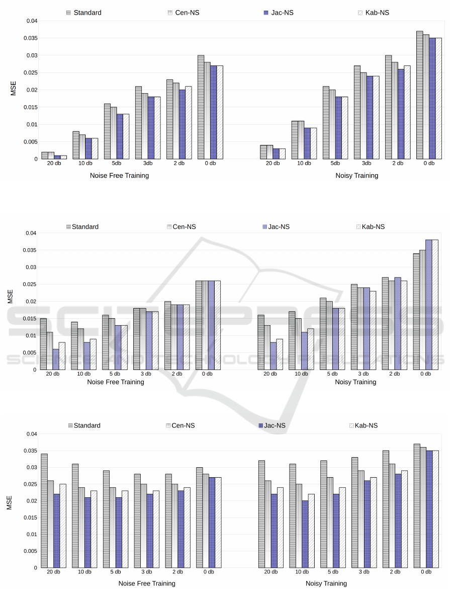
Figure 7: The NSFLS Prediction performance comparison produced by different inference based approaches. Each standard

deviation of input FSs is set to the corresponding noise level.

Figure 8: The NSFLS Prediction performance comparison. Each standard deviation of input FSs is set to 5 dB σ

noise

Figure 9: The NSFLS Prediction performance comparison. Each standard deviation of input FSs is set to 0 dB σ

noise

4 CONCLUSION AND FUTURE

WORK

We have implemented and compared different infer-

ence based approaches (Standard, cen-NS, jac-NS,

and Kab-NS). Because of the limitations and issues

observed in current approaches, this paper has fo-

cused on exploring the potential of a new novel sim-

ilarity measure in combination with the similarity

based inferencing approach. Kabir’s similarity mea-

sure (Kabir et al., 2017) is sensitive both to changes

in the width of FSs and to the case in which one FS

is a subset of another. Considering these features, it

has now been used for the ﬁrst time to deﬁne ﬁring

levels in FLSs. The evidence from this study points

towards the idea that similarity based inferencing ap-

proach with the Kabir’s similarity measure could in-

deed be a suitable approach to be used in FLSs. How-

ever, this is a tentative ﬁnding, and more work needs

to be carried out on different data sets under a wider

range of conditions to further evaluate this.

Future work will concentrate on different inter-

esting aspects. The similarity based inferencing ap-

proach will be implemented by using different sim-

ilarity measures (e.g. Dice similarity) between an-

tecedents and input FSs. Alternative time series

datasets (for example, the Lorenz time series) will

be used in FLS. Different design types for antecedent

and input FSs will be implemented and the results will

be examined. Lastly, due to the increased modelling

capabilities of type-2 fuzzy logic in handling uncer-

tainty, different type-2 designs will be explored.

ACKNOWLEDGEMENTS

This research was supported by a University of Not-

tingham (School of Computer Science) Postgraduate

Studentship.

REFERENCES

Balazinski, M., Czogala, E., and Sadowski, T. (1993). Con-

trol of metal-cutting process using neural fuzzy con-

troller. In Fuzzy Systems, 1993., Second IEEE Inter-

national Conference on, pages 161–166. IEEE.

Hayashi, Y., Buckley, J. J., and Czogala, E. (1993). Fuzzy

neural network with fuzzy signals and weights. Inter-

national Journal of Intelligent Systems, 8(4):527–537.

Jaccard, P. (1908). Nouvelles recherches sur la distribution

ﬂorale.

Kabir, S., Wagner, C., Havens, T. C., Anderson, D. T., and

Aickelin, U. (2017). Novel similarity measure for

interval-valued data based on overlapping ratio. In

2017 IEEE International Conference on Fuzzy Sys-

tems (FUZZ-IEEE 2017).

Larsen, P. M. (1980). Industrial applications of fuzzy logic

control. International Journal of Man-Machine Stud-

ies, 12(1):3–10.

Mackey, M. C., Glass, L., et al. (1977). Oscillation and

chaos in physiological control systems. Science,

197(4300):287–289.

Mamdani, E. H. and Assilian, S. (1975). An experiment

in linguistic synthesis with a fuzzy logic controller.

International journal of man-machine studies, 7(1):1–

13.

McCulloch, J. and Wagner, C. (2016). Measuring the

similarity between zslices general type-2 fuzzy sets

with non-normal secondary membership functions. In

IEEE World Congress on Computational Intelligence

(WCCI 2016).

Mendel, J. M. (2001). Uncertain rule-based fuzzy logic sys-

tems: introduction and new directions. Prentice Hall

PTR Upper Saddle River.

Mouzouris, G. C. and Mendel, J. M. (1997). Nonsingleton

fuzzy logic systems: theory and application. IEEE

Transactions on Fuzzy Systems, 5(1):56–71.

Pedrycz, W. (1992). Design of fuzzy control algorithms

with the aid of fuzzy models. Industrial Applications

of Fuzzy Control, 12(1):153–173.

Pourabdollah, A., Wagner, C., and Aladi, J. (2015).

Changes under the hood - a new type of non-singleton

fuzzy logic system. In 2015 IEEE International Con-

ference on Fuzzy Systems (FUZZ-IEEE), pages 1–8.

Sahab, N. and Hagras, H. (2010). A hybrid approach

to modeling input variables in non-singleton type-2

fuzzy logic systems. In 2010 UK Workshop on Com-

putational Intelligence (UKCI), pages 1–6.

Wagner, C., Pourabdollah, A., McCulloch, J., John, R.,

and Garibaldi, J. M. (2016). A similarity-based in-

ference engine for non-singleton fuzzy logic systems.

In 2016 IEEE International Conference on Fuzzy Sys-

tems (FUZZ-IEEE), pages 316–323.

Wang, L.-X. and Mendel, J. M. (1992). Generating fuzzy

rules by learning from examples. IEEE Transactions

on systems, man, and cybernetics, 22(6):1414–1427.

Zadeh, L. A. (1965). Fuzzy sets. Information and control,

8(3):338–353.