Investigation of Three Immiscible Fluids in a Microchannel
Accounting for the Pressure Gradient and the Electroosmotic Flow
Nicolas La Roche-Carrier, Guyh Dituba Ngoma, Fouad Erchiqui and Ibrahim Hamani
School of Engineering’s Department, University of Quebec in Abitibi-Témiscamingue,
445, Boulevard de l’Université, Rouyn-Noranda, Quebec, J9X 5E4, Canada
Keywords: Immiscible Fluids, Microchannel, Modeling and Simulation.
Abstract: This study deals with the investigation of three immiscible fluids in a microchannel consisting of two parallel
plates. These fluids were composed of two electric conducting fluids and one electric nonconducting fluid.
The concept of pumping a nonconducting fluid using interfacial viscous shear stress was applied accounting
for the effect of the electroosmosis and pressure gradient. The electric potential and the flow parameters were
found resolving the Poisson-Boltzmann equation and the modified Navier-Stokes equations for a hydraulic
steady fully-developed laminar flow of an incompressible fluid. The results achieved revealed the influence
of the wall and interfacial zeta potentials, the pressure difference, and the dynamic fluid viscosity ratio on the
flow characteristics of the three immiscible fluids. The developed approach was compared with a model of
two immiscible flows to highlight the relevance of this work.
1 INTRODUCTION
Microfluidic transport is widely used in the fields of
micropumps, micropower generation, chemical
processes, biomechanical processes and heat transfer,
where surface effects dominate the flow behavior
within microdevices (Dituba Ngoma G. et al., 2005).
The precise knowledge of the immiscible fluids flow
behavior in microchannels is essential to develop
high-performance microfluidic devices to pump a
nonconducting fluid by means of conducting fluids.
This can be achieved taking relevant fluid parameters
and microchannel configurations into consideration
in the planning, design and optimization phases. Most
previous investigations of pressure gradient and
electroosmotic flow in microchannels were
performed using a single conducting fluid with the
zeta potentials at the microchannel walls (Dhinakaran
S. et al., 2010; Vainshtein P. et al., 2002; and Brask
A. et al., 2005). There, the effects of surface potential,
electric field, ionic concentration and channel size on
the velocity distribution and the effect of friction on
flow characteristics. Furthermore, Yong et al., 2011
numerically analyzed the immiscible kerosene-water
two-phase flows in microchannels connected by a T-
junction using lattice Boltzmann method. In addition,
Dituba Ngoma G. et al., 2005; and Gao Y. et al., 2005,
conducted a study on two immiscible fluids
consisting of a conducting fluid and a nonconducting
fluid in a microchannel. The electric field and the
pressure gradient were applied. Moreover, an
analytical model of mixed electroosmotic/pressure
driven three immiscible fluids in a rectangular
microchannel was developed by Li H. et al., 2009.
They analyzed the effects of viscosity ratio,
electroosmosis and pressure gradient on velocity
profile and flow rate. Thorough analysis of previous
works clearly demonstrated that the research results
obtained are specific to the microchannel
configuration depending on considered key
parameters of fluids and microchannels. Therefore,
in this work, to enhance the fluid flow of
nonconducting fluids and performances of the flow in
microchannels, an investigation was conducted
considering the fluid flow of the three immiscible
fluids in a two parallel plates to deeply analyze the
impacts of the zeta potential, the pressure difference
and the dynamic viscosity on the flow characteristics
of the three fluids.
428
Roche-Carrier, N., Ngoma, G., Erchiqui, F. and Hamani, I.
Investigation of Three Immiscible Fluids in a Microchannel Accounting for the Pressure Gradient and the Electroosmotic Flow.
DOI: 10.5220/0006481004280433
In Proceedings of the 7th International Conference on Simulation and Modeling Methodologies, Technologies and Applications (SIMULTECH 2017), pages 428-433
ISBN: 978-989-758-265-3
Copyright © 2017 by SCITEPRESS – Science and Technology Publications, Lda. All rights reserved

2 MATHEMATICAL
FORMULATION
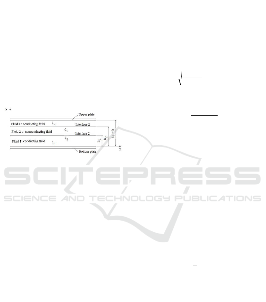
The model of three immiscible fluids in two parallel
plates considered in this study is shown in Fig. 1. The
two plates separated by a distance h. The
microchannel is filled of two electric conducting
fluids, the fluid 1 and the fluid 3, and one non-
conducting fluid, the fluid 2. These fluids have
different dynamic viscosities which are specified by
µ
1
, µ
2
, and µ
3
, respectively. The interface positions
are specified using the heights h
1
and h
2
. The forces
acting on the conducting fluids include the pressure
force and the electric body force generated by the
double layer electric field. For the non-conducting
fluid, only the pressure force acts on this.
Figure 1: Model of three immiscible fluids.
To develop the governing equations for the liquid
flow of the three immiscible fluids in a microchannel
accounting for the electroosmosis, the following
assumptions were made: (i) A steady state, one-
dimensional and laminar flow was assumed; (ii) no-
slip boundary conditions were assumed; (iii) a planar
interface between the immiscible fluids was assumed;
(iv) the fluid shear stress and the flow velocity were
the same at the fluid interface; (v) the fluids were
assumed to be incompressible; and (vi) the gravity
effect was negligible.
2.1 Electric Potential Field
According to the electrokinetic (Dituba Ngoma G. et
al., 2005; and Li H. et al., 2009), the equation of the
electric potential of ions, , in y direction for the
conducting fluids is given as:
0
e
2
2
dy
d




. (1)
where  is the dielectric constant of the solution, 
0
the permittivity of vacuum, and 
e
the net charge
density.
The net charge density can be written assuming a
symmetric electrolyte as:
,
Tk
ez
sinhezn2
b
0
0e










(2)
where e, k
b
, n

, T and z
0
are the elementary charge,
Boltzmann constant, bulk concentration of ions,
absolute temperature and valence of ions,
respectively.
Combining the Eqs. 1 and 2, and using the Debye-
Hückel approximation, Eq. 3 is found:
,
dy
d
2
2
2


(3)
where
Tk
n2
ez
b0
0



is the Debye-Hückel
parameter and

1
is the Debye length.
The net charge density Eq. 2 can be rewritten as:




Tk
ezn2
b
22
0
e
. (4)
Introducing the Debye-Hückel parameter in Eq. 4, the
last can be expressed by:

2
0e
. (5)
To solve Eq. 3, the following boundary conditions for
the conducting fluids are used:
0 y 
1
hy
2
hy 
3
hy 
1

for the bottom wall,
2

for the interface of the fluids
1 and 2,
3

for the interface of the
fluids 2 and 3,
4

for the upper wall.
(6)
Using the dimensionless parameters and variables,
Eq. 3 can be formulated as:
*2
2*
*2
K
dy
d


. (7)
where
,
Tk
ez
b
0
*


,
h
y
y
*

,hK 
h is the distance
between the plates, it equal to h
3
.
The boundary conditions of Eq. (7) in dimensionless
form can be written as for the conducting fluid “fluid
1”:
0 *y 
*
1
h *y 
*
1
*

,
*
2
*

.
(8)
For the conducting fluid “fluid 3”. They are expressed
by:
*
2
*
hy 
1hy
*
3
*

*
3
*

,
*
4
*

.
(9)
Investigation of Three Immiscible Fluids in a Microchannel Accounting for the Pressure Gradient and the Electroosmotic Flow
429

Where
,
h
h
h
1
*
1

,
h
h
h
2
*
2

,1
h
h
h
3
*
3

,
Tk
ez
b
10
*
1


,
Tk
ez
b
30
*
3


.
Tk
ez
b
40
*
4


In addition, the net charge density in dimensionless
form is given by:
ezn
0
e
*
e



.
(10)
When considering the expression of
*
, Eq. 10
becomes:
*
*
e
2
.
(11)
The solutions of Eqs. 7 and 11 can be written as:
,BeAe*
*Ky*Ky 

 
.BeAe2
*Ky*ky*
e


(12)
where A and B are determined accounting for the
boundary conditions. In general case, these boundary
conditions can be expressed as follows:
*
i
*
hy 
*
j
*
hy 
*
i
*

,
*
j
*

.
(13)
Substituting Eq. 13 for * in Eq. 12, Eq. 14 is found
*
i
*
i
KhKh
*
i
BeAe


,
*
j
*
j
KhKh
*
j
BeAe


.
(14)
From Eq. 14, A and B are determined:
,
ee
ee
A
)hh(K)hh(K
Kh
j
Kh
i
*
j
*
i
*
j
*
i
*
i
*
j






.
ee
ee
B
)hh(K)hh(K
Kh
j
Kh
i
*
j
*
i
*
j
*
i
*
i
*
j




(15)
Furthermore, for the conducting fluids “fluid 1”
and “fluid 2”, A and B are calculated using Eq. 16:
0h
*
i

*
1
*
j
hh 
*
2
*
i
hh 
1h
*
j

*
1
*
i

,
,
*
2
*
j

,
*
3
*
i

.
*
4
*
j

(16)
2.2 Hydrodynamic Field
The modified Navier-Stokes equations for the fluids
1, 2, and 3 can be expressed by:
,E
y
u
P0
e
2
3
2
3x




,E
y
u
P0
e
2
1
2
1x




.
y
u
P0
2
2
2
2x



(17)
where
dx
dp
P
x

assuming that the pressure gradient
in x direction is constant. E and E
e
are the electric
field and the electric body force, respectively.
Eq. 17 represents three second-order differential
equations. Thus, six boundary conditions are required
in order to solve them. The no-slip boundary
conditions can be written as based on Fig.1:
0)0y(u
1

,
0)hy(u
33

.
(18)
Moreover, the boundary conditions for the same
velocity at the interfaces of the fluids 1 and 2, and the
fluids 2 and 3 can be formulated as follows:
)hy(u)hy(u
1211

,
)hy(u)hy(u
2322

.
(19)
In addition, the boundary conditions for the
interfacial shear stresses are described as:
,
y
u
y
u
11
hy
2
2
hy
1
1







.
y
u
y
u
22
hy
3
3
hy
2
2







(20)
Solving Eq. 17 accounting for the boundary
conditions, the dimensionless velocities are
determined:
,ayaC
2
yC
u
2
*
1
*
1
2*
0
*
1

,byb
2
yC
u
2
*
1
2*
4
*
2

.ayaC
2
yC
u
4
*
3
*
3
2*
2
*
3

(21)
where
0
1
*
1
u
u
u 
,
0
2
*
2
u
u
u 
,
0
3
*
3
u
u
u 
, u
0
is an arbitrary
reference velocity,
,
u
Ph
C
01
x
2
0


,
u
u
C
0
1h
1

,
u
Ph
C
03
x
2
2


,
u
u
C
0
3h
3

and
.
u
Ph
C
02
x
2
4


u
h1
and u
h3
are the Helmholtz-
SIMULTECH 2017 - 7th International Conference on Simulation and Modeling Methodologies, Technologies and Applications
430

Smoluchowski electroosmotic velocities for the
conducting fluids “fluid 1” and “fluid 3”,
respectively. They are given by:
10
b0
1
h
ez
TKE
u



and
30
b0
3h
ez
TKE
u



.
(22)
The dimensionless boundary conditions can be
formulated as:
 
,00*yu
*
1

   
,huhu
*
1
*
2
*
1
*
1

   
,huhu
*
2
*
3
*
2
*
2

 
,01hu
*
3
*
3

,
y
u
y
u
*
1
**
1
*
hy
*
*
2
hy
*
*
1






,
y
u
y
u
*
2
*
*
2
*
hy
*
*
3
hy
*
*
2








(23)
where
1
2



and
1
3



.
Accounting for the boundary conditions Eq. 23, the
system of six equations in matrix form are found in
order to determine the constants a
1
,a
2
,a
3
,a
4
,b
1
and
b
2
:
6x1 6x1 6x6
,
G
G
G
G
G
G
b
b
a
a
a
a
0 - 0 0 0
0 - 0 0 0 1
1- h- 1 h 0 0
1- h- 0 0 1 h
0 0 1 1 0 0
0 0 0 0 1 0
6
5
4
3
2
1
2
1
4
3
2
1
*
2
*
2
*
1
*
1

































































(24)
where:
,C G
*
111

,C
2
C
G
*
43
2
2

,
2
hC
C
2
hC
G
2*
14
*
21
2*
10
3

,
2
hC
C
2
hC
G
2*
24
*
33
2*
22
4

,eBeAKC
hChCG
*
1
*
1
Kh
1
Kh
11
*
10
*
145









.eBeAKC
hChCG
*
2
*
2
Kh
3
Kh
33
*
24
*
226









(25)
2.3 Dimensionless Flow Rates
The flow rate between the parallel plates is
determined by integrating the flow velocity
distribution over the cross-sectional area. For the
fluids 1, 2, and 3, the dimensionless flow rates are
expressed respectively by:
,1eB1eA
K
C
hah
2
a
h
6
C
Q
*
1
*
1
Kh
1
Kh
1
1
*
12
2
*
1
1
3
*
1
0
*
1
























 
 
,hhb
2
hh
b
6
hhC
Q
*
1
*
22
2*
1
2*
2
1
3*
1
3*
24
*
2













     
.eeBeeA
K
C
h1ah1
2
a
h1
6
C
Q
*
2
*
2
Kh
K
3
Kh
K
3
3
*
24
2*
2
3
3*
2
2
*
3

























(26)
3 NUMERICAL RESULTS AND
DISCUSSION
Numerical simulations were done using the
MATLAB software to investigate and analyze the
effects of the wall and interfacial zeta potentials, the
pressure difference, the interface position, the
dynamic viscosity ratio on flow characteristics of the
three immiscible fluids in a microchannel between
two plates. The main reference data for all simulation
runs in this study are given as: 
0
= 8.854 x 10
-12
C/(m
V),  = 80, n
∞
= 6.022 x 10
20
1 m³, z
0 = 1
, E =15000 V/m ,
T = 298 K, k
b
= 1.381 x 10
-23
J/K, 
1
= 0.001 Pa s,  = 1 ,
 = 1, L = 0.02 m, and u
0
=1 m/s.
3.1 Impact of the Zeta Potential
To analyze the impact of the zeta potential on the
electric potential for the conducting fluids “fluid 1”
and “fluid 3”, all parameters were kept constant
except the wall, and interfacial zeta potentials. Fig. 2
shows the dimensionless electric potential as a
function of the dimensionless height of the fluid with
the dimensionless wall and the interfacial zeta
potentials as parameters. There, it can be seen that the
effect of the zeta potential is very pronounced on the
microchannel bottom and upper walls, and the
interface positions of the three fluids. The electric
potential is zero for the nonconducting “fluid 2”.
Investigation of Three Immiscible Fluids in a Microchannel Accounting for the Pressure Gradient and the Electroosmotic Flow
431

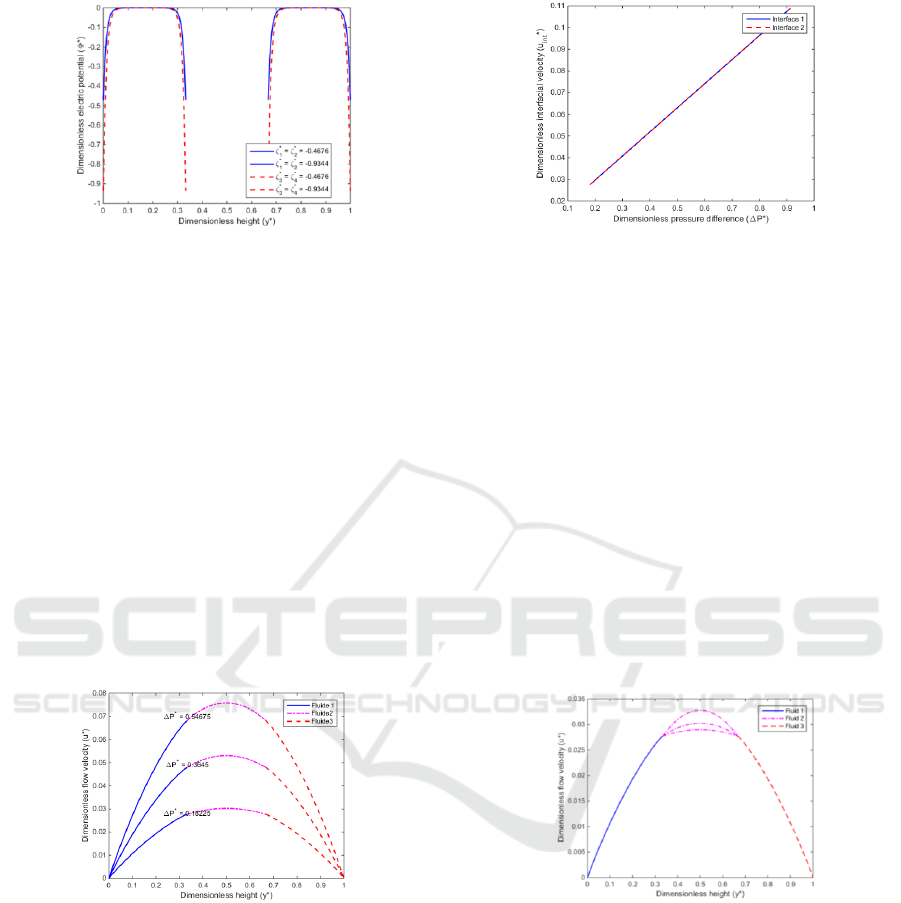
Figure 2: Dimensionless electric potential versus
dimensionless height.
3.2 Impact of the Pressure Difference
To investigate the impact that the pressure difference
in a microchannel has on the flow velocity, the
dynamic viscosity ratios, the wall zeta potentials, the
interfacial zeta potentials, the interface positions; the
pressure differences were varied using the
dimensionless values. Fig. 3 shows the dimensionless
flow velocity distribution in the microchannel cross-
section. From this figure, it can be observed that the
dimensionless flow velocities for the three
immiscible fluids increase when the dimensionless
pressure difference between the microchannel inlet
and outlet increases. This well explain the pumping
of the nonconducting fluid “fluid 2” by means of two
conducting fluids “fluid 1” and “fluid 3”.
Figure 3: Dimensionless flow velocity versus
dimensionless height.
Moreover, Fig. 4 represents the dimensionless
interfacial flow velocity for the three fluids as a
function of the dimensionless pressure difference,
where it can be seen that the dimensionless interfacial
flow velocity increases with the dimensionless
pressure difference.
Figure 4: Dimensionless interfacial flow velocity versus
dimensionless pressure difference.
3.3 Impact of the Dynamic Viscosity
Ratio
To examine the effect of the dynamic viscosity ratio
“” between the fluids 1 and 2 on the interfacial flow
velocity, and the flow velocity; all parameters were
kept constant, except the dynamic viscosity ratio “”.
Fig. 5 shows the distribution of the dimensionless
flow velocity for the three fluids as a function of the
dimensionless height of the fluid with the dynamic
velocity ratio ““ as parameter. From this figure, it
can be seen that the dimensionless flow velocities for
the three fluids decrease when the dynamic viscosity
ratio “ “ increases. This can be explained by the fact
that the resistance to fluid flow increases when the
dynamic viscosity of a fluid increases.
Figure 5: Dimensionless flow rate versus dimensionless
height.
3.4 Model Comparison
The developed model of the three immiscible fluids
in microchannel consisting of two parallel plates was
compared with the model of two immiscible fluids in
two parallel plates (Dituba Ngoma G. et al., 2005).
The results obtained shows that the maximum
dimensionless velocity was achieved for the model of
three fluids as depicted in Fig. 6. That highlights the
relevance to consider the concept of two conducting
fluids to drive a conducting fluid.
SIMULTECH 2017 - 7th International Conference on Simulation and Modeling Methodologies, Technologies and Applications
432

a) Model of two immiscible fluids
b) Model of three immiscible fluids
Figure 6: Model comparison.
4 CONCLUSION
In this work, a model of the flow of three immiscible
fluids in a microchannel formed by two parallel plates
was investigated. The concept of pumping an electric
nonconducting fluid using two electric conducting
fluids was applied. The combined effect of the
pressure gradient and electroosmosis was accounted
for to identify the flow parameters that improve the
flow of the nonconducting fluid. Based on the
modified Navier-Stokes and the Poisson-Boltzmann
equations, numerical simulations were accomplished.
The results obtained demonstrate that, among other
things, the dynamic viscosity ratios, the zeta
potentials and the pressure difference affects the flow
behavior in a microchannel in a strong yet different
manner. A comparison between the developed
approach of three fluids and a model of two fluids was
done to show the relevance of this study.
REFERENCES
Dhinakaran S., Afonso A.M., Alves M.A., Pinho F.T. 2010.
Steady viscoelastic fluid flow between parallel plates
under electro-osmotic forces: Phan-Thien–Tanner
model. Journal of Colloid and Interface Science 344,
513–520.
Vainshtein P. and Gutfinger C. 2002. On electroviscous
effects in microchannels. J. Micromech. Microeng. 12,
252-256.
Brask A., Goranovic G., Jensen M. J. and Bruus H., A,
2005. Novel electro-osmotic pump design for
nonconducting liquids: theoretical analysis of flow
rate–pressure characteristics and stability, J.
Micromech. Microeng. 15, 883-891.
Yong Y., Yang C., Jiang Y., Joshi A., Shi Y. and Yin X.,
2011. Numerical simulation of immiscible liquid-liquid
flow in microchannels using lattice Boltzmann method.
Science China Chemistry, Vol.54 No.1: 244–256.
Gao Y., Wong T. N., Yang C., Ooi K. T., 2005. Two-fluid
electroosmotic flow in microchannels. Journal of
Colloid and Interface Science 284 (2005) 306-314.
Dituba Ngoma G., Erchiqui Fouad, 2005. Pressure gradient
and electroosmotic effects on two immiscible fluids in
a microchannel between two parallel plates, Journal of
Micromechanics and Microengineering 16, 83–91.
Li H., Teck N. W., Nam-Trung N., 2009. Analytical model
of mixed electroosmotic/pressure driven three
immiscible fluids in a rectangular microchannel.
International Journal of Heat and Mass Transfer 52,
4459-4469.
Investigation of Three Immiscible Fluids in a Microchannel Accounting for the Pressure Gradient and the Electroosmotic Flow
433