
Re-optimisation Control of a Fed-batch Fermentation Process using
Bootstrap Aggregated Extreme Learning Machine
Carolina Maria Cardona Baron and Jie Zhang
School of Chemical Engineering and Advanced Materials, Newcastle University, Newcastle upon Tyne NE1 7RU, U.K.
Keywords: Fed-Batch Processes, Fermentation, Neural Networks, Extreme Learning Machine, Re-optimisation.
Abstract: This paper presents using bootstrap aggregated extreme learning machine for the on-line re-optimisation
control of a fed-batch fermentation process. In order to overcome the difficulty in developing mechanistic
model, data driven models are developed using extreme learning machine (ELM). ELM has the advantage
of fast training in that the hidden layer weights are randomly assigned. A single ELM model can lack of
robustness due the randomly assigned hidden layer weights. To overcome this problem, multiple ELM
models are developed from bootstrap re-sampling replications of the original training data and are then
combined. In addition to enhanced model accuracy, bootstrap aggregated ELM can also give model
prediction confidence bounds. A reliable optimal control policy is achieved by means of the inclusion of
model prediction confidence bounds within the optimisation objective function to penalise wide model
prediction confidence bounds which are associated with uncertain predictions as a consequence of plant
model-mismatch. Finally, in order to deal with process disturbances, an on-line re-optimisation strategy is
developed and successfully implemented.
1 INTRODUCTION
The production of Saccharamyces cervisia
commonly called baker’s yeast follows a
fed-batch fermentation process. The massive
consumption of this product results in a competitive
market, making the maximization of biomass
production a key target to be achieved. The
complexity of the fermentation processes dynamics
makes this a non-trivial and challenging but also
very interesting optimisation problem.
The challenges that are faced in the optimal
control of biochemical processes comprise the
modelling of highly non-linear systems,
characterisation of those kinds of processes, and the
development of a reliable control policy capable of
providing good performance under plant model
mismatch. On one side, mechanistic models are
usually very difficult to be developed, due to the
complex dynamics of the growing microorganisms.
Therefore, data-driven modelling techniques based
on process operation data have been recently
developed to provide accurate solutions for process
modelling (Chen et al., 1995; Tian et al., 2002).
Nevertheless, typically the collection of process
operational data is limited, in part because of the
highly costs involved in the experiments for data
acquirement, coupled with the physical limitation to
measure certain key process variables.
Therefore, in the last decades, data-driven
modelling techniques based on neuronal networks
have been widely accepted as they can provide an
effective way to build accurate models based on
process operation data (Tian et al., 2001; Zhang et
al., 1997; Zhang and Morris, 1999; Zhang, 2005).
Certainly, the leading advantage of neural networks
is their ability to model complex non-linear
processes, which is perhaps achieved through their
parallel structure, which provides them with
excellent capabilities to store knowledge. It is not a
coincidence that neural networks resembles the
human brain in the sense that knowledge is learnt
from observations and stored in the form of inter-
neural connection strengths Noor et al. (2010).
Typically, neural network performance can be
affected by over fitting of the training data and their
generalization capabilities can be seriously
compromised, resulting in considerable prediction
errors when unseen data is presented to the network.
Furthermore, the speed of learning process is also
concerned, since typically the training process with
traditional feedforward training algorithms is very
Baron, C. and Zhang, J.
Re-optimisation Control of a Fed-batch Fermentation Process using Bootstrap Aggregated Extreme Learning Machine.
DOI: 10.5220/0006477601650176
In Proceedings of the 14th International Conference on Informatics in Control, Automation and Robotics (ICINCO 2017) - Volume 1, pages 165-176
ISBN: 978-989-758-263-9
Copyright © 2017 by SCITEPRESS – Science and Technology Publications, Lda. All rights reserved
165

slow, because all the parameters of the network need
to be tuned. Therefore, to address those common
drawbacks, a novel algorithm developed by Huang
et al. (2006), called Extreme Learning Machine
(ELM), provides an extremely fast learning speed,
coupled with better generalization capabilities in
comparison to traditional learning algorithms. In
ELM some of the network parameters are randomly
chosen, reducing the computational efforts in
network training. However, single ELM models may
lack robustness and give varying performance due to
the hidden layer weights are randomly assigned. To
address this issue, the idea of bootstrap aggregated
neural networks (Zhang, 1999) can be used in
developing bootstrap aggregated ELM. The use of
bootstrap aggregated neural networks is widely
recognized as an effective method to reduce the lack
of robustness in the models that is caused principally
due to over-fitting, enhancing the model
generalization capabilities (Ahmad and Zhang,
2006; Xiong and Zhang, 2005; Zhang et al., 2006;
Osuolale
and Zhang, 2017).
In the last decade, a reliable optimisation strategy
based on bootstrap aggregated neural network
models has been proposed by Zhang (2004), in
which a reliable optimal control policy is obtained
by means of the inclusion of model prediction
confidence bounds within the objective function of
the optimisation problem. The modified optimisation
objective function penalises wide model prediction
confidence bounds. In this way, an optimal control
can be successfully implemented in the actual
process without suffering from performance
degradation, which is commonly caused by plant-
model mismatch.
The rest of the paper is organised as follows.
Section 2 presents a feed-batch fermentation
process. Section 3 presents bootstrap aggregated
ELM. Modelling of the feed-batch fermentation
process using bootstrap aggregated ELM is
presented in Section 4. Section 5 presents reliable
optimisation control of the feed-batch fermentation
process. Both off-line optimisation and on-line re-
optimisation control are presented. Finally, Section 6
draws some concluding remarks.
2 A FED-BATCH
FERMENTATION PROCESS
The fed-batch fermentation process uses Baker’s
yeast as the basis reactant and the kinetic and
dynamic model is taken from (Yuzgec et al., 2009),
which gives a dynamic model based on mass
balance equations described by glucose, ethanol,
oxygen and biomass concentrations. The kinetic
model is represented by the following 12 equations
(Yuzgec et al., 2009):
Glucose uptake rate:
=
,
+
1−
(1)
Oxidation capacity:
,
=
,
+
+
(2)
Specific growth rate limit:
,
=
/
(3)
Oxidative glucose metabolism:
,
=
,
,
/
⁄
(4)
Reductive glucose metabolism:
,
=
−
,
(5)
Ethanol uptake rate:
,
=
,
+
+
(6)
Oxidative ethanol metabolism:
,
=
,
,
−
,
/
/
(7)
Ethanol production rate:
,
=
,
/
(8)
Total specific growth rate:
=
,
/
+
,
/
+
,
/
(9)
Carbon dioxide production rate:
=
,
/
+
,
/
+
,
/
(10)
Oxygen consumption rate:
=
,
/
+
,
/
(11)
Respiratory Quotient:
=
⁄
(12)
The mass balance equations describe the
dynamic of glucose, ethanol, oxygen and biomass
concentrations as follows (Yuzgec et al., 2009):
ICINCO 2017 - 14th International Conference on Informatics in Control, Automation and Robotics
166

=
−
−
/
+
,
/
+
(13)
=−
+
∗
−
−
(14)
=
,
−
,
−
(15)
=
−
(16)
= (17)
=113
.
(18)
where C
s
, C
o
, C
e
, and C
x
represent, respectively, the
concentrations of glucose, oxygen, ethanol and
biomass, F and F
a
stand for feed rate and air feed
rate respectively, and A
R
denotes the cross-sectional
area of the reactor. The other symbols and values of
model parameters are given in Tables 1 and 2.
Table 1: Definition of process variables and parameters.
k
L
ao total volumetric mass transfer coefficient (h
-1
)
K
e
saturation constant for ethanol (gL
-1
)
K
i
inhibition constant (gL
-1
)
K
o
saturation constant for oxygen (gL
-1
)
K
s
saturation constant for substrate (gL
-1
)
Y
i/j
yield of component i on j (gg
-1
)
V volume (L)
μ specific growth rate (h
-1
)
Superscripts and subscripts:
* interface
cr critic
e ethanol
lim limitation
o oxygen
ox oxidative
pr production
red reductive
s substrate (glucose)
up uptake
x biomass
Based on the mechanistic model, a simulation
programme is developed in MATLAB. The
simulation programme is used to generate process
operational data and to test the developed models
and optimisation control policies. The batch initial
conditions considered for the simulation are taken
from (Yuzgec et al., 2009) and are summarized as
follows:
Initial conditions:
0
=
7gL
;
0
=7.8
gL
;
0
=
0gL
;
0
=15gL
;
0
=50000
Volume of the fermentor V
=100
Concentration of feed S
=
325
Final time: t
=16.5ℎ
Table 2: Numeric values of the parameters in the fed-batch
model.
K
e
0.1 gL
-1
Yx/e 0.7187 gg
-1
K
i
3.5 gL
-1
Qe,max 0.238 gg
-1
h
-1
K
o
9.6×10
-5
gL
-1
Qo,max 0.255 gg
-1
h
-1
K
s
0.612 gL
-1
Qs,max 2.943 gg
-1
h
-1
OX
SX
Y
/
0.585 gg
-1
Q
m
0.03 gg
-1
h
-1
red
SX
Y
/
0.05 gg
-1
S
o
325 gh
-1
Y
o/s
0.3857 gg
-1
*
o
C
0.006 gh
-1
Y
o/e
0.8904 gg
-1
A
R
12.56 m
2
Y
e/s
0.4859 gg
-1
μ
cr
0.21 h
-1
Y
e/o
1.1236 gg
-1
3 BOOTSTRAP AGGREGATED
EXTREME LEARNING
MACHINES
3.1 Extreme Learning Machine
Feedforward neural networks are very useful to
model complex non-linear systems and are capable
to estimate the relationships between process
variables just by learning from the training data
presented to the network through the execution of a
learning algorithm. Although the development of
neural network models is significantly more
practical and easier to implement than the classical
mathematical modelling approaches, the time
required to train neural networks using traditional
learning algorithms is considerably high, making the
learning a slow process (Huang et al., 2006).
Huang et al. (2006) mention that the attention of
researchers has been dedicated to the generalization
capabilities of neural networks using finite training
data sets. However, the training process typically
involves the tuning of all network parameters, i.e.
weights and biases, and in many cases requires
iterative computations until acceptable performance
has been achieved. To reduce the computational
burden in neural network training, Huang et al.
(2006) propose the ELM, a novel learning algorithm
for single hidden layer feedforward networks
(SLFN) in which some of the network parameters
are chosen randomly, reducing significantly the
learning speed while achieving good generalization
capabilities.
Re-optimisation Control of a Fed-batch Fermentation Process using Bootstrap Aggregated Extreme Learning Machine
167

Figure 1: A single hidden layer feedforward network.
The algorithm proposed by Huang et al. (2006) is
described as follows: a SLFN is built from distinct
pair of samples
,
with
=
,
,…,
∈
and
=
,
,…,
∈
. The SLFN has Ñ hidden neurons. The th
neuron in the hidden layer is connected with the
input layer through a weighting vector,
=
,
,…,
, and has activation function
and bias
. At the output layer, nodes are connected
through the weighting vector
=
,
,…,
that links the th hidden neuron with the output
nodes, which have a linear activation function.
=
∙
+
=
Ñ
Ñ
=1,2,…,
(19)
As long as the SLFN with
infinitely
differentiable can learn distinct observations,
which can be written as
∑
−
=0
Ñ
, then it
should exist a finite value for
,
,
that meet the
following:
∙
+
=
Ñ
=1,2,…,
(20)
The relationship given in Eq(20) can be written
in matrix notation as Eq(21), where is called the
hidden layer output matrix:
=
(21)
,…,
Ñ
,
,…,
Ñ
,
,…,
=
∙
+
⋯
Ñ
∙
+
Ñ
⋮⋱⋮
∙
+
⋯
Ñ
∙
+
Ñ
Ñ
(22)
=
⋮
Ñ
Ñ
and =
⋮
(23)
Then, the proposed algorithm (Huang et al.,
2006) suggests setting the parameters
,
randomly and compute the matrix H. Following that,
the remaining unknown variable in Eq(21) is only
the vector , which can be found as:
=
(24)
In the above equation,
corresponds to the
Moore-Penrose generalized inverse of the matrix ,
which can be found through several methods; for
instance, the orthogonal projection, singular value
decomposition (SVD), orthogonalization method
and iterative method. The last two methods are
avoided since iterations are undesired because can
increase the computation times of the ELM
algorithm. Instead, if
is non-singular, the
orthogonal projection method can be used, so
=
. Whereas, in many cases the matrix
tends to be singular, the SVD method performs
well under those circumstances.
3.2 Bootstrap Aggregated ELM
In the light of the techniques to develop the multiple
neural networks, Noor et al. (2010) identifies three
basic kinds of stacked neural networks, in which the
individual networks are combined using a particular
method. The first type is the multiple model neural
networks, characterized for using different training
data to build the individual networks; hence, training
data can relate to different inputs and include
information about a wider operation region. This
approach also allows different training algorithms
for each network. Conversely, the second category
employs the same data to train the individual
networks, but re-sampled or divided according to
one of the following algorithms: bootstrap re-
sampling (Efron, 1982), adaboost or ‘adaptive
boosting’ or randomisation. Finally, the third
category involves a selective combination of neural
networks, in order to reduce the error induced by
networks with poorest generalization capabilities.
With this in mind, the scope of this work is centred
in bootstrap aggregated ELM, known as BA-ELM.
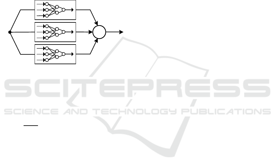
As is mentioned by Zhang (1999), the principle
of stacked neural networks, shown in Figure 2, is to
develop several neural networks to model the same
relationship. Hence, model generalization capability
and accuracy can be improved as a result of a proper
combination of all networks, instead of just selecting
the “best” single neural network. The overall output
of a BA-ELM, expressed in Eq(1), is a weighted
combination of the individual networks outputs.
O
1
x
n
x
2
x
1
1
2
Ñ
...
β
11
Inpu
t
L
ayer Ou
t
pu
t
layer
...
1
m
...
β
1m
β
Ñ1
β
Ñm
O
m
Hidden layer
β
21
β
2m
activation function: g(x) activation function: linear
ICINCO 2017 - 14th International Conference on Informatics in Control, Automation and Robotics
168
=
(25)
where,
is the BA-ELM predictor,
is the
th ELM,
is the aggregating weight for the th
ELM, is the vector of inputs and is the number
of ELM models. The selection of weighting
parameters is fundamental to achieve good
performance. In general, the simple approach taking
equal weights is enough to attain enhanced results.
However, aggregating weights can also be computed
using principal component regression (PCR), since it
is less sensitive to highly correlated data, which is
the case for the individual networks.
Figure 2: Bootstrap aggregated ELM.
Finally, an advantage in using BA-ELM is that
confidence bounds for model predictions can be
calculated from the individual network estimations
as follows (Zhang, 1999):
=
1
−1
;
−
;∙
⁄
(26)
where
corresponds to the standard error of the th
predicted value,
;∙
=
∑
;
⁄
and
is the number of ELM models. Under the
assumption that prediction errors are normally
distributed, the 95% prediction confidence bound
can be found as
;∙
±1.96
. Thus, more
reliable predictions are associated with small values
of
.
4 PROCESS MODELLING USING
BOOTSTRAP AGGREGATED
ELM
4.1 Data Generation and
Pre-Processing
Simulated process operational data were generated
from simulation. In total, 75 batches were simulated.
The feed profiles of these batches were obtained by
adding random variations to a base feed profile. The
batch time in divided into 17 equal intervals and the
substrate feed rate is kept constant in each interval.
Thus the feed profile can be represented by a vector
of 17 elements. The ELM model is of the following
form:
y=f(x
1
, x
2
, …, x
17
) (27)
where y is the biomass concentration at the end of a
batch, x
1
to x
17
are the substrate feed rates over a
batch.
Data pre-processing is carried out to remove
undesired information such as noise, outliers, non-
representative samples, etc. Data pre-processing
tools include for example normalization to scale the
data, filtering to cope with measurement noise,
removing trends and outliers to eliminate
inconsistent data that potentially will lead to wrong
results, etc.
4.2 BA-ELM Modelling
Once the data have been scaled to unity variance and
zero mean in the previous step, 80% (60 batches) of
data are selected for model building and the
remaining 20% (15 batches) are left as the unseen
validation data. Then, the original training set is here
re-sampled using bootstrap re-sampling with replace-
ment (Efron, 1982) to produce =50 different
bootstrap replication sets, which are going to be used
to train each one of the individual neural networks.
Specifically, the bootstrap re-sampling is a simple
technique in which, random samples (batches) from
the original data are picked. As a consequence, some
samples can be picked more than once and some may
not be picked at all. In this way, the learning informa-
tion presented to each network is slightly different,
which is the powerful concept of BAGNET (Zhang,
1999), since the networks do not learn exactly the
same information, they can complement to each other.
Figure 3 shows model predictions on the 15
unseen batches (validation data) and their respective
confidence bounds. It can be seen that the model
predictions are reasonably accurate. The SSE of the
individual networks on training and validation data
are shown in Figure 4. In general, from the graph it
can be seen that network performance on training data
is not always consistent with the performance on the
unseen validation data, since a network with a small
SSE value on the training data can have a large SSE
value on the validation data or vice versa, thus it is
evident that a single neural network is not robust
enough to produce accurate predictions.
x
ŷ
Σ
Re-optimisation Control of a Fed-batch Fermentation Process using Bootstrap Aggregated Extreme Learning Machine
169
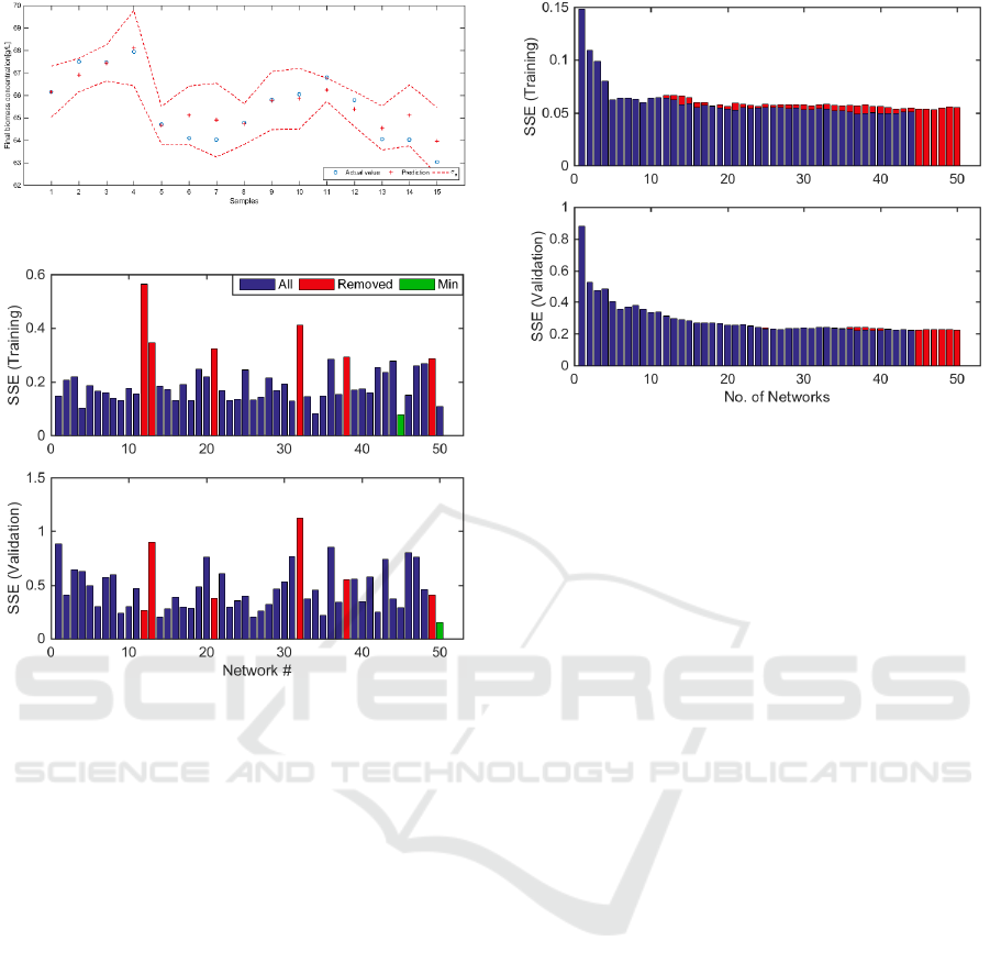
Figure 3: Model predictions on validation data.
Figure 4: Model errors of individual networks.
Furthermore, the networks highlighted in colour
red in Figure 4 were removed from the stacked
network, under the criterion of being the worst
performing on training data. However, only 6 were
chosen because bad performing on training data does
not necessarily imply also poor performance on
unseen data; for instance, networks #12 and #21
were in the worst group, but those networks actually
have good performance on validation data. For this
reason, it is not advisable to remove a lot of those
bad performing networks, because some of those can
produce quite accurate results on validation data.
Conversely, the networks #13, #32 and #38
performed bad in both cases, thus it is appropriate to
remove the influence of those networks. Highlighted
in colour green, the minimum SSEs on training data
was 0.0767 due to the network #45, and 0.1501 for
validation data due to the network #50.
On the other hand, Figure 5 clearly shows the
advantage of stacking multiple neural networks.
Figure 5 shows the model performance of
aggregating different numbers of ELM, from 1 (the
first single ELM) to 50 (aggregating all 50 ELM
models). It shows the SSE values of BA-ELM with
different numbers of ELM models on the training
Figure 5: Model error of stacked networks.
and validation data. Thus, the highest error in both
cases occurs, as is expected, when just one network
produces the predicted value. Then, the error is
significantly reduced while more networks are being
combined. It is important to notice the consistent
pattern of SSE reduction on the training data and the
validation data. Additionally, the influence of the
removed networks can be seen in colour red, which
corresponds to the SSEs before those networks were
eliminated. Before removing the worst networks, the
minimum SSEs on training data was 0.0530 with the
contribution of 47 networks, and 0.2207 for
validation data with 28 networks added. After
removing the bad performing networks, the values
decrease to 0.0492 with the contribution of 37
networks on training data, and 0.2191 for validation
data with 37 networks added. On balance, the SSEs
were reduced in both training and validation data
just by means of an arrangement of multiple non-
robust models.
5 PROCESS OPTIMISATION
USING BOOTSTRAP
AGGREGATED ELM
5.1 Off-line Optimisation
The operation objective of the fed-batch
fermentation process is to produce as much product
as possible. Here the objective function J is defined
in terms of the neural network model, and
particularly in this study, the width of the model
prediction confidence bounds is included to improve
ICINCO 2017 - 14th International Conference on Informatics in Control, Automation and Robotics
170

the reliability of the optimal control policy. The
optimisation problem can be written as follows:
min
=−
+
:
0≤≤3000
ℎ
⁄
≤
=100000
(28)
where
is the BAGNET output, which
specifically corresponds to the predicted biomass
concentration at the end of the batch
, =
,
,…,
is the vector of substrate feed rates
divided in hourly intervals;
is the standard error
of model prediction, and is a penalty factor for
.
Operational constraints are imposed, for instance,
the feed flow rate is bounded to maximum 3000
[L/h] and the volume of the total biomass is
restricted by the fermenter volume
. This objective
function is aimed to maximise the amount of product
while minimise the width of the model prediction
confidence bounds to achieve a reliable optimal
control policy.
The optimisation problem given in Eq(28) was
solved using the Interior-Point algorithm, available
in Matlab
®
Optimisation Toolbox, which is an
effective non-linear programming method, specially
for constrained problems.
Different values of were considered, in order to
analyse the influence of penalising wide model
prediction confidence bounds. Then, the optimal
control policy obtained for all the cases was applied
to the mechanistic model based simulation to
evaluate the performance. The results are presented
in Table 3, which contains the value of biomass
given by the mechanistic model, the neural network
prediction and the confidence bound
, for each
value of .
Specifically, the first entry in Table 3
corresponds to =0, which is equivalent to the
optimisation problem without considering the
confidence bounds in the objective function, in other
words, the unreliable control policy. In that case, the
neural network prediction for the final biomass was
75.788 [g/L] while the actual value (from
mechanistic model) was significantly lower 51.583
[g/L], and
=0.182. The notable difference
between the model prediction and the actual value is
in fact what motivated the researchers to include the
confidence bounds into the objective function, since
as has been evidenced, an optimal control policy on
the model can lead to poor performance when
applied to the actual process due to plant model
mismatches.
Thus, the value of was increased gradually in
order to analyse the effect of the penalisation term in
the objective function. Consequently, as is shown in
Table 3 with =1 a considerable improvement of
the actual value of biomass was achieved (59.544
[g/L]), which of course also results in the reduction
of the
to 0.167. After trying with further values of
, the actual final biomass concentration reached
71.236 [g/L] when =12, and the confidence
bounds were reduced to half its initial value; at the
same time, the neural network prediction decrease to
75.409 [g/L]. Therefore, from Table 3 it is possible
to appreciate that by means of increasing the
penalisation of wide model prediction confidence
bounds, the optimal substrate feeding profile
becomes more reliable, since the performance on the
actual process is not degraded.
Nevertheless, as the value of increases, the
meaning on the objective function in Eq(4) is to give
more importance to the reduction of the
, which as
a consequence, will sacrifice the maximisation of the
final product concentration. Therefore, there is an
inherently conflict between the two terms in the
objective function. Thus, while the error becomes
smaller, the maximisation term is reduced, as well as
the actual biomass. To make clear that point, further
values of were tried, corresponding to the last two
columns of Table 3; for =120, the value of
was notably reduced as well as the relative error
between the model prediction and the actual value.
However, this was achieved with a reduction in the
final biomass production. For this reason, the value
of =12 is selected as the optimal weighting
factor, since it offers a balance between both
objectives.
Table 3: Final biomass concentrations and
with respect
to λ.
λ
Mechanistic
model
BA-ELM
σ
e
0 51.583 75.788 0.182
1 59.544 75.781 0.167
2 65.733 75.763 0.155
3 68.959 75.739 0.145
5 70.203 75.682 0.130
6 70.521 75.650 0.125
9 71.163 75.520 0.107
12 71.236 75.409 0.096
45 71.163 74.549 0.059
120 70.943 72.702 0.036
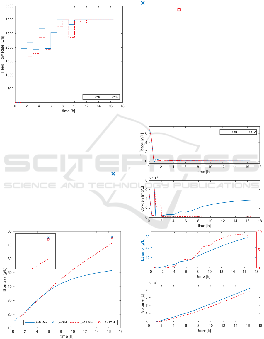
Figure 6 shows the optimal feeding profiles
which correspond to the ‘unreliable’ optimal control
policy when =0 (continuous blue line) and the
improved profile when =12 (red dashed line).
Figures 7 and 8 present the profiles of biomass,
glucose, oxygen, ethanol and volume when the
Re-optimisation Control of a Fed-batch Fermentation Process using Bootstrap Aggregated Extreme Learning Machine
171
optimal substrate feeding profile is applied to the
process, which is in fact the simulation of the
mechanistic model.
Figure 6: Optimisation results: Control Policy.
Figure 7 shows the actual biomass profile and the
prediction value of the neural network. From this
figure, it is absolutely evident the poor performance
obtained with the unreliable control policy
(continuous blue line), since the final biomass
concentration value of 51.583 [g/L], is quite far from
the target prediction by the neural network ( ) of
75.788 [g/L]. Conversely, with the feeding profile
when=12 (red dashed line), although the final
value 71.236 [g/L], was not exactly the same as that
predicted by the neural network 75.409[g/L], the
control policy is more reliable since it is shown to
have good performance on the actual process. The
small box at the top left of the graph is a zooming
Figure 7: Optimisation results: Biomass.
window that shows closely the final value of
biomass with the enhanced profile, and shows that
the target without considering the confidence bounds
( ) was slightly higher than the target given by the
reliable profile ( ).
Moreover, Figure 8 shows the concentrations of
glucose, oxygen, ethanol and the reaction volume.
Particularly, it is interesting to analyse the ethanol
formation, since is considerably high when =0,
with a final concentration around 30 [g/L], which is
perhaps what is causing the drop of the final biomass
concentration. It must be remembered that, Ethanol
formation is undesirable, since is a by-product that
can deteriorate the amount and quality of the
product. Thus, the reliable control profile obtained
when =12, gives better performance because the
ethanol formation is successfully reduced to
concentrations around 10 [g/L]. Although this is not
directly included in the objective function, it is
implicitly related with the confidence bounds. In
other words, increasing the penalization of wide
Figure 8: Optimisation results: Glucose, Oxygen, Ethanol,
and Volume.
ICINCO 2017 - 14th International Conference on Informatics in Control, Automation and Robotics
172

other words, increasing the penalization of wide
confidence bounds, the optimisation algorithm tries
to find an optimal profile closer to the knowledge of
the network, which was trained with data with
reduced ethanol concentration. Therefore, the
optimal control policy is more reliable also in the
sense that it tries to generate a control policy that is
well known by all the individual networks.
5.2 On-line Re-optimisation
In a realistic scenario, besides plant model
mismatch, disturbances can also lead to poor
performance of the process when the optimal profile
is applied. To cope with this situation, the on-line re-
optimisation strategy (Xiong and Zhang, 2005) is
implemented by means of taking on-line
measurements of the process every 4 hours and re-
estimating the optimal control profile for the
remaining batch period.
Initially, the optimal profile is calculated off-line
for the complete batch time
=
,
,…,
,
which corresponds to the optimal profile found
earlier with =12. The process is operated with the
first two values f
1
and f
2
of
applied to the process
(mechanistic model based simulation). Then, when
two hours have elapsed, a measurement of the
process is taken and, a new optimal profile ids re-
calculate for the remaining stages in the batch,
which now starts from the third interval, and the
result is given as
=
,
,…,
. Then, the
process is fed with the new
,
,
,
, and 4
hours later the process is measured again. Similarly,
a new optimal profile is estimated but now starting
from the seventh interval
=
,
,…,
; just
,
,
,
are actually used because at the
end of tenth interval the process is measured once
again, and another re-optimised profile is found
=
,
,…,
; 4 hour later the last re-
optimisation is executed and the batch is finished
with this profile
=
,
,
.
In order to perform the re-optimisations, it is
necessary to develop four neural network models
that include as inputs the process measurements and
the feeding profile considering just the appropriate
feeding intervals. Of course, all the networks are
aimed to predict the biomass concentration at the
end of the batch. Therefore, the new BA-ELM
models can be written as follows:
=
2
,
, where
2
is the
biomass concentration measurement at =
2ℎ and
=
,
,…,
are the feed
flow rate intervals in
/ℎ
.
=
6
,
, where
6
is the
biomass concentration measurement at =
6ℎ and
=
,
,…,
are the feed
flow rate intervals in
/ℎ
.
=
10
,
, where
10
is the
biomass concentration measurement at =
10ℎ and
=
,
,…,
are the feed
flow rate intervals in
/ℎ
.
=
14
,
, where
14
is the
biomass concentration measurement at =
14ℎ and
=
,
,
are the feed
flow rate intervals in
/ℎ
.
Once the four neural networks were developed, the
process was simulated but a disturbance was
introduced by modifying one of the mechanistic
model parameters. The initial substrate
concentration
was change from its nominal value
of 325 gL
to 305 gL
, to pretend an unknown
behaviour of the process and validate the on-line
optimisation strategy.
From Table 4 it can be observed that, by means
of updating the control policy, taking measurements
of the process, was possible to modify the initial
deviation of the process due to the disturbance, to
achieve the same final biomass concentration as was
obtained with the reliable off-line profile. The neural
network prediction for the on-line case in Table 4 is
given by the fourth neural network. Moreover, it is
natural that, although the fourth neural network is
the most accurate of all, an error between the actual
process and the network prediction occurs, since the
process is under the effect of disturbance and the
neural network was not trained to learn any
observation with that kind of mismatch. However,
what is important rather than the error in the
prediction is that the target final biomass was
modified and reached a closer value to the desired
target.
Table 4: Final biomass concentration.
Off-line On-line
Mechanistic model 71.236 –
Model+disturbance 67.4971 71.1244
Neural Network 75.409 73.7741
Re-optimisation Control of a Fed-batch Fermentation Process using Bootstrap Aggregated Extreme Learning Machine
173
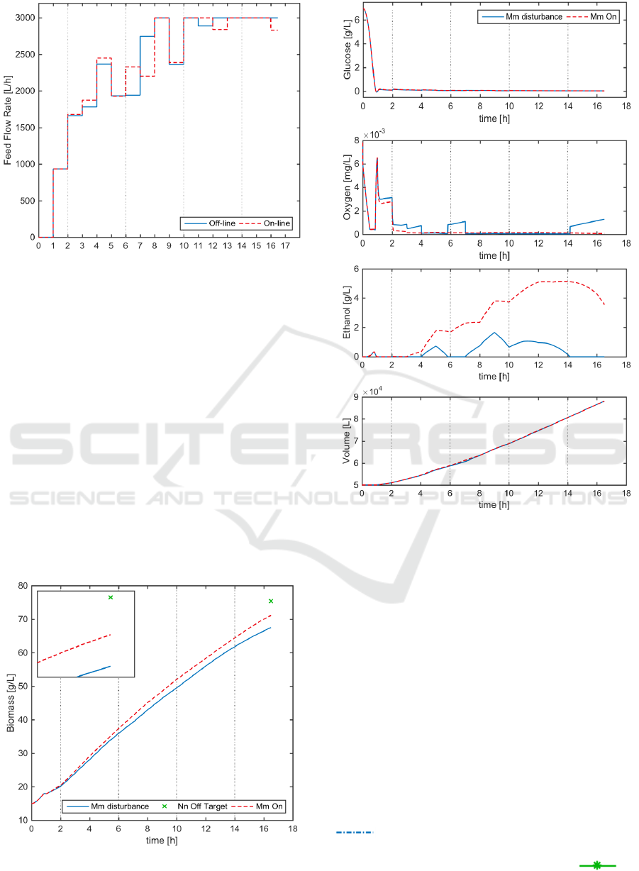
Figure 9: On-line Optimisation results: Control Policy.
To illustrate the results obtained, Figure 9 shows
the initial control policy calculated off-line
(continuous blue line) and the re-optimised profile
(dashed red line), which was updated every four
hours starting in the second hour, according to the
division lines in the graph. Figure 10 shows the
biomass concentration profile, where it can be seen
that the first two hours both profiles are equal, since
no re-calculation has been performed. After the
second hour, the feed flow rate is successfully
modified to drive the biomass concentration towards
the desired optimal value. The small box at the top
left corner is a zooming window that illustrates
closely the difference of the off-line control policy
applied on the process under disturbance
(continuous blue line) and the successful modified
profile (dashed red line).
Figure 10: On-line Optimisation results: Biomass.
Figure 11: On-line Optimisation results: Glucose, Oxygen,
Ethanol, Volume.
Figure 11 shows the overall process
performance, represented by the concentrations of
glucose, oxygen, ethanol and volume profiles. With
respect to ethanol concentration, there is an extra
amount of ethanol production, when the on-line re-
optimisation is performed, which perhaps is due to
the efforts to achieve the biomass production target,
since the substrate feed rate remains in the upper
bound most of the time after the 10
th
interval.
Finally, as an illustration of the control policy re-
calculations during the batch that lead to the optimal
feeding profile previously shown in Figure 8 (dashed
red line), Figure 12 contains all the re-optimised
profiles and highlights the time interval that is
actually applied to the process with a thick line. For
example, the off-line control policy denoted as
(
) is just applied for the first two hours, which
are represented with a thick line. Then, after the
second hour, the new optimal profile
() is
applied for the next four hours. Then, again a new
ICINCO 2017 - 14th International Conference on Informatics in Control, Automation and Robotics
174
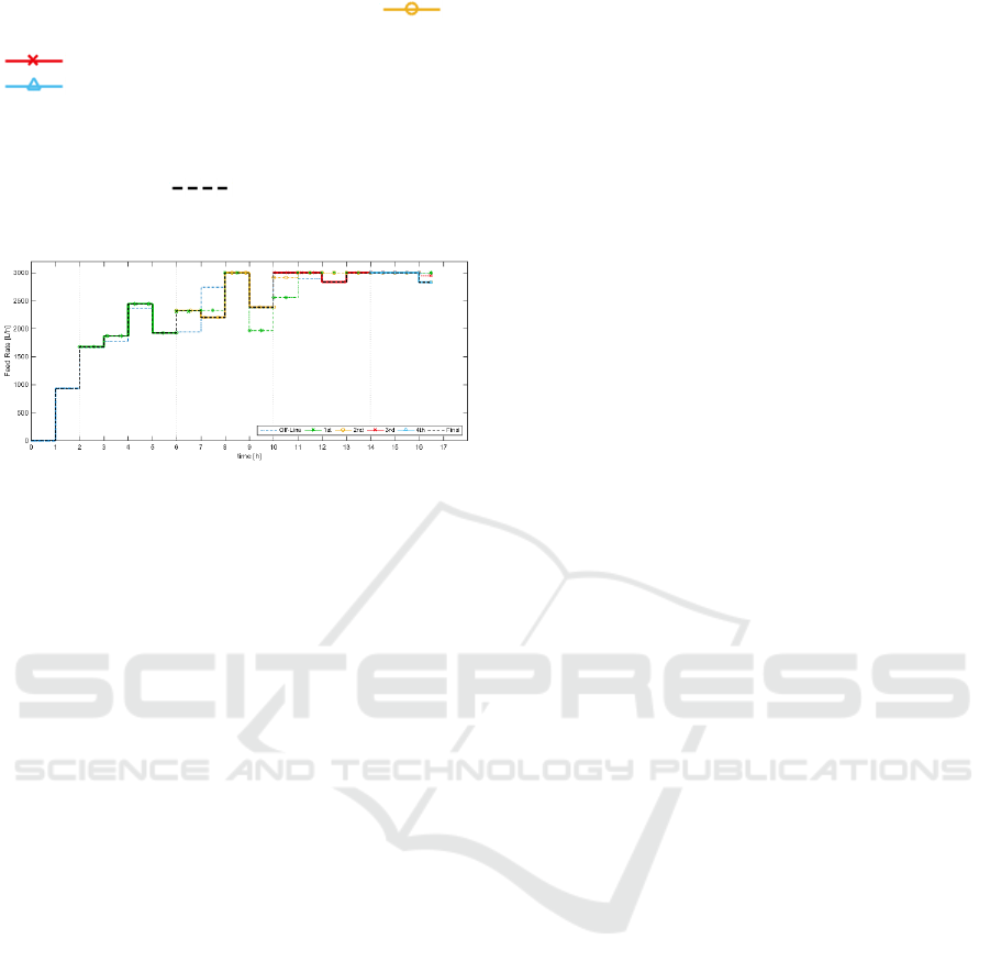
re-calculation is made, and the profile
() is
applied for four hours, when is replaced by
(
). The last re-optimisation corresponds to
(
), which is entirely applied, since it is the
ending period of the batch. Consequently, although
all the feeding profiles are calculated for the entire
batch time, the resulting optimal profile, which is
denoted as
( ) is built just with the first
four intervals of each is profile.
Figure 12: On-line Optimisation results: Detailed Control
Policy.
6 CONCLUSIONS
Modelling and reliable optimisation control of a fed-
batch fermentation process using bootstrap
aggregated extreme learning machine (BA-ELM) is
studied in this paper. It is shown that aggregating
multiple ELM models can enhance model prediction
performance. As the training of each ELM is very
quick, building BA-ELM models does not have
computation issues. The model prediction
confidence bound of BA-ELM model is
incorporated in the optimisation objective so that the
reliability of the calculated optimal control policy
can be enhanced. In order to overcome the
detrimental effect of unknown disturbances, on-line
re-optimisation is carried out to update the off-line
calculated optimal control policy. Applications to a
simulated fed-batch fermentation process
demonstrate the effectiveness of the proposed
modelling and reliable optimisation control
technique.
ACKNOWLEDGEMENTS
The work was supported by the EU (Project No.
PIRSES-GA-2013-612230) and National Natural
Science Foundation of China (61673236).
REFERENCES
Ahmad, Z., Zhang, J. 2006. Combination of multiple
neural networks using data fusion techniques for
enhanced nonlinear process modelling. Computers &
Chemical Engineering, 30(2), 295-308.
Chen, L., Zhang, J., Morris, A. J., Montague, G. A., Kent,
C. A., Norton, J. P. 1995. Combining neural networks
with physical knowledge in modelling and state
estimation of bioprocesses. Proceedings of the 3rd
European Control Conference, Rome, Italy, 5-8
September, 1995, 2426-2431.
Efron, B. 1982. The Jacknife, the Bootstrap and Other
Resampling Plans. Philadelphia: Society for Industrial
and Applied Mathematics.
Huang, G.-B., Zhu, Q.-Y., Siew, C.-K. 2006. Extreme
learning machine: Theory and applications.
Neurocomputing, 70, 489-501.
Noor, R. A. M., Ahmad, Z., Don, M. M., Uzir, M. H.
2010. Modelling and control of different types of
polymerization processes using neural networks
technique: A review. The Canadian Journal of
Chemical Engineering, 88, 1065-1084.
Osuolale, F., Zhang, J. 2017. Thermodynamic
optimization of atmospheric distillation unit.
Computers & Chemical Engineering, 103, 201-209.
Tian, Y., Zhang, J., Morris, A. J. 2001. Modelling and
optimal control of a batch polymerisation reactor using
a hybrid stacked recurrent neural network model. Ind.
Eng. Chem. Res. 40(21), 4525-4535.
Tian, Y., Zhang, J., Morris J. 2002. Optimal control of a
fed-batch bioreactor based upon an augmented
recurrent neural network model. Neurocomputing,
48(1-4), 919-936.
Xiong, Z., Zhang, J. 2005. Neural network model-based
on-line re-optimisation control of fed-batch processes
using a modified iterative dynamic programming
algorithm. Chemical Engineering and Processing:
Process Intensification, 44, 477-484.
Xiong, Z., Zhang, J. 2005. Optimal control of fed-batch
processes based on multiple neural networks. Applied
Intelligence, 22(2), 149-161.
Yuzgec, U., Turker, M., Hocalar, A. 2009. On-line
evolutionary optimization of an industrial fed-batch
yeast fermentation process. ISA Trans, 48, 79-92.
Zhang, J., Morris, A. J., Martin, E. B., Kiparissides, C.
1997. Inferential estimation of polymer quality using
stacked neural networks. Computers & Chemical
Engineering, 21, s1025-s1030.
Zhang, J. 1999. Developing robust non-linear models
through bootstrap aggregated neural networks.
Neurocomputing, 25, 93-113.
Zhang, J., Morris, A. J. 1999. Recurrent neuro-fuzzy
networks for nonlinear process modelling. IEEE
Transactions on Neural Networks, 10(2), 313-326.
Zhang, J. 2004. A reliable neural network model based
optimal control strategy for a batch polymerization
reactor. Industrial and Engineering Chemistry
Research, 43, 1030-038.
Re-optimisation Control of a Fed-batch Fermentation Process using Bootstrap Aggregated Extreme Learning Machine
175

Zhang, J. 2005. Modelling and optimal control of batch
processes using recurrent neuro-fuzzy networks. IEEE
Transactions on Fuzzy Systems, 13(4), 417-427.
Zhang, J., Jin, Q., Xu, Y. M. 2006. Inferential estimation
of polymer melt index using sequentially trained
bootstrap aggregated neural networks. Chemical
Engineering and Technology, 29(4), 442-448.
ICINCO 2017 - 14th International Conference on Informatics in Control, Automation and Robotics
176
