Exploiting Optical Flow Field Properties for 3D Structure Identification
Tan Khoa Mai
1
, Michèle Gouiffès
2
and Samia Bouchafa
1
1
IBISC, Univ. d’Evry Val d’Essonne, Université Paris Saclay, France
2
LIMSI, CNRS, Univ. Paris Sud, Université Paris Saclay, F-91405 Orsay, France
Keywords:
Optical Flow, C-velocity, 3-D Plane Reconstruction.
Abstract:
This paper deals with a new method that exploits optical flow field properties to simplify and strengthen the
original c-velocity approach (Bouchafa and Zavidovique, 2012). C-velocity is a cumulative method based
on a Hough-like transform adapted to velocities that allows 3D structure identification. In case of moving
cameras, the 3D scene is assumed to be composed by a set of 3D planes that could be categorized in 3 main
models: horizontal, lateral and vertical planes. We prove in this paper that, by using directly pixel coordinates
to create what we will call the uv-velocity space, it is possible to detect 3D planes efficiently. We conduct our
experiments on the KITTI optical flow dataset (Menze and Geiger, 2015) to prove our new concept besides
the effectiveness of uv-velocity in detecting planes. In addition, we show how our approach could be applied
to detect free navigation area (road), urban structures like buildings and obstacles from a moving camera in
the context of Advanced Driver Assistance Systems.
1 INTRODUCTION
Advanced driver assistance systems are one of the
fastest growing markets in the world
1
thanks to the
constant development in security and intelligence of
autonomous vehicles which has been the outcome of
many works in this domain. For trajectory and obsta-
cles detection tasks, ADAS systems are widely based
on multi-sensors cooperation (Lidar, accelerometers,
odometers, etc.) rather than on computer vision.
However, data fusion from different sensors is not
straightforward since sensors always provide impre-
cise and missing information. Moreover, most of
these sensors are very specialized and provide limited
information while vision can be used for many tasks
like: scene structure analysis, motion analysis, recog-
nition, and so on. Even if stereovision appears widely
preferred in this context, it is very restrictive because
of camera calibration or/and rectification step(s) (Lu
et al., 2004). We propose to focus in our study on
"monocular" vision for its several advantages includ-
ing its cost, both economic and energetic, and the
wealth of information extracted from monocular im-
age sequences like (among others) obstacle motion.
Among all existing monocular approaches, we
chose to focus on the c-velocity method (Bouchafa
1
https://www.mordorintelligence.com/industry-
reports/advanced-driver-assistance-systems-market
and Zavidovique, 2012) because of its potential ro-
bustness. This method is based on the exhibition of
constant velocity loci whose pattern is bound to the
orientation of planes to be detected (e.g. horizon-
tal or vertical). Velocities obtained from an optical
flow technique are cumulated in the c-velocity space.
Thanks to its cumulative nature, c-velocity has the ad-
vantage to be very robust toward optical flow impre-
cision. In the classical c-velocity approach, a voting
space is designed for each plane category. Our study
aims at detecting 3-D planes in image sequences by
proposing a more efficient formulation of the original
c-velocity approach. We consider the case where im-
ages are captured from a camera on-board a moving
vehicle and deal with urban scenes. Unlike other 3-D
reconstruction methods that require camera calibra-
tion (Lu et al., 2004), our method called "uv-velocity"
offers, under few assumptions, a more generic way to
reconstruct the 3D scene around the autonomous ve-
hicle without any calibration. Many studies for ADAS
applications deal with estimating egomotion of cam-
eras (Luong and Faugeras, 1997; Azuma et al., 2010),
detecting free navigable space (roads) or obstacles
(Oliveira et al., 2016; Mohan, 2014), (Cai et al., 2016;
Ren et al., 2017). The uv-velocity can do all of them
without any learning algorithm.
In (Labayrade et al., 2002), the authors propose a
method to detect the horizontal plane by using a new
Mai, T., Gouiffès, M. and Bouchafa, S.
Exploiting Optical Flow Field Properties for 3D Structure Identification.
DOI: 10.5220/0006474504590464
In Proceedings of the 14th International Conference on Informatics in Control, Automation and Robotics (ICINCO 2017) - Volume 2, pages 459-464
ISBN: Not Available
Copyright © 2017 by SCITEPRESS – Science and Technology Publications, Lda. All rights reserved
459

Figure 1: Coordinates system in case of a moving camera.
histogram called the v-disparity map. Their work
has inspired many works in lanes and obstacles de-
tection for autonomous vehicles (Soquet et al., 2007;
Qu et al., 2016). The c-velocity is the transposi-
tion of the v-disparity concept to motion: instead of
stereo camera, c-velocity deals with monocular vi-
sion. The idea behind the c-velocity is that, under
a pure translation of the camera, the norm w of a ve-
locity vector of a moving plane (estimated using an
optical flow method) varies linearly with a pixel value
that is called the c-value (or c). The latter is com-
puted from only pixels position on the image plane.
As in both the v-disparity method and in the classi-
cal Hough transform, 3D planes should be detected
thanks to a line detection process in the c-velocity vot-
ing space. A re-projection is done to associate to each
pair (c,w), its corresponding set of pixels in the im-
age. In the original c-velocity method, this process is
not optimized since the estimation of two intermedi-
ate variables (c,w) is required and involve square root
and power operations. However, in practice, obtained
results from the c-velocity method confirms its reli-
ability in real condition. Using the same methodol-
ogy and assumptions than the c-velocity method, we
find out that using only u or v components of the ve-
locity vectors instead of the norm to create suitable
voting spaces leads to more intuitive characteristics
that make easier plane model interpretation. More-
over, we show that this new formulation can keep the
performance of detections as well. The uv-velocity
is more similar to the v-disparity than the c-velocity
if we try to find an analogy. A tough problem like
detecting horizontal 3D planes (resp. vertical planes)
becomes - using the v-velocity (resp. u-velocity) - a
simple parabola curve detection process in the defined
voting space. Frontal planes (assimilated to obstacles
in the 3D scene) can be detected in these two voting
spaces by finding straight lines. After finding these
curves in the voting space thanks to a Hough trans-
form, we re-project the v-y or u-x back to the image
to reveal planes.
The paper is organized as follows: section 2 ex-
plains mathematically the chosen models and presents
all required equations. Section 3 explains how to
build the voting space and provides information about
the curve detection process. Section 4 shows results
of our uv-velocity method for detecting 3D planes.
Section 5 discusses the results and provides some
ideas for future work.
2 MAIN ASSUMPTIONS AND
MODELS
This section details the chosen camera coordinates
system and gives the 2D projection of a 3-D plane
motion. We assume that the 2D motion in the im-
age could be approximated by the optical flow. We
consider three relevant plane models in case of urban
scenes: horizontal, lateral and vertical.
One can suppose an image sequence taken from
a camera mounted on a moving vehicle. The optical
axis of the camera is aligned with Z (see Fig.1).
Two frame coordinates are considered: OXY Z for
representing 3-D points in real the 3D scene and oxy
for representing the projection of these points on the
image plane. A 3D point P(X ,Y,Z) is projected on
the image plane at point p(x,y) using the well-known
projection equations: x = f
X
Z
and y = f
Y
Z
, where f is
the focal length of the sensor.
In case of a moving camera, with a translational
motion T = [T
X
,T
Y
,T
Z
]
T
and a rotational motion
Ω = [Ω
X
,Ω
Y
,Ω
Z
]
T
, according to (Bouchafa and Zavi-
dovique, 2012), 2D motion vectors of pixels belong-
ing to a 3D plane could be expressed as:
u =
xy
f
Ω
X
−

x
2
f
+ f

Ω
Y
+ yΩ
Z
+
xT
Z
− f T
X
Z
v = −
xy
f
Ω
Y
+

y
2
f
+ f

Ω
X
+ xΩ
Z
+
yT
Z
− f T
Y
Z
(1)
2D motion vectors converge to a unique location in
the image. This particular point, which depends on
the translational motion, is called the Focus of Ex-
pansion (FOE) and its coordinates are given by:
x
FOE
=
f ×T
X
T
Z
and y
FOE
= −
f ×T
Y
T
Z
(2)
In case of a pure translational motion, (1) be-
comes:
u =
xT
Z
− f T
X
Z
and v =
yT
Z
− f T
Y
Z
(3)
A 3D plane is characterized by its distance d to the
origin O and its normal vector n = [n
X
,n
Y
,n
Z
]
T
, with
equation: |n
X
X + n
Y
Y + n
Z
Z| = d. All points visible
by the camera have Z > 0. By dividing plane equa-
tion by Z and combining with projection equations,
we get:
1
f d
|n
X
x + n
Y
y + n
Z
f | =
1
Z
(4)
ICINCO 2017 - 14th International Conference on Informatics in Control, Automation and Robotics
460

Replacing Z in Eq.3 by Z in Eq.4, 2D motion of a
3D plane is:
u =
1
f d
|n
X
x + n
Y
y + n
Z
f |(x T
Z
− f T
X
)
v =
1
f d
|n
X
x + n
Y
y + n
Z
f |(yT
Z
− f T
Y
)
(5)
Since the translational motion T = [T
X
,T
Y
,T
Z
]
T
,
the focus f of the camera and the distance d are con-
stant for a given plane, the Eq.5 represents the rela-
tion between the pixels coordinates and the 2D mo-
tion assimilated to the optical flow. Using this rela-
tion, planes can be easily detected without knowing
neither the egomotion nor the intrinsic parameter f of
the camera.
In urban scenes, without any loss of generality,
three main plane models (horizontal, vertical, lat-
eral) can be considered. They are characterized by
their normal vectors: [0,1,0]
T
for Horizontal planes,
[0,0,1]
T
for Vertical planes and [1,0,0]
T
for Lateral
planes. By injecting these normal vector values into
Eq.5, the equation is declined into the three formu-
lations given in Table.1. These equations reveal two
terms: one of them depends only on pixel positions (it
is called the c-value), the second one depends on the
egomotion, the focal length and the plane-to-origin
distance.
Table 1: 2D motion equations for three main plane models:
horizontal, vertical and lateral.
Planes u v
Horizontal
T
Z
f d
r
|y|(x −x
FOE
)
T
Z
f d
r
|y|(y −y
FOE
)
Vertical
T
Z
d
o
(x −x
FOE
)
T
Z
d
o
(y −y
FOE
)
Lateral
T
Z
f d
b
|x|(x −x
FOE
)
T
Z
f d
b
|x|(y −y
FOE
)
In the original c-velocity method, the norm w =
√
u
2
+ v
2
of a velocity vector and the c-value are used
to create a 2D voting space where one of the axis is
w and the other is c. Since there is a linear relation-
ship between them in case of moving planes, detect-
ing lines in the c-velocity space is equivalent to detect
3D planes:
w =
T
Z
f d
r
y
2
q
(x −x
FOE
)
2
+ (y −y
FOE
)
2
= K ×c
(6)
where c = y
2
p
(x −x
FOE
)
2
+ (y −y
FOE
)
2
. Lines in
the c-velocity space are detected using a classical
Hough transform. In our case, we chose to consider
separately the two components of a velocity vector.
Each component could be exploited to detect a spe-
cific plane model. Let us study each of them sepa-
rately in the following subsections.
2.1 Horizontal Plane Model
In practice, in the context of ADAS, an horizontal
plane represents the road on which the vehicle moves.
For sake of simplicity, without compromising with re-
ality, according to our model assumptions, road pix-
els are always located under the y
FOE
in the image
and the vertical position sign does not change for the
whole road. From Table. 1, we have:
u = K
r
y(x −x
FOE
)v = K
r
y(y −y
FOE
) (7)
where K
r
= sign(y)
T
Z
f d
r
. If |u|=constant (or
|v|=constant), from Eq.7, we can draw the iso-motion
contours on the image. These contours show wher-
ever the pixels have the same component u(v) if they
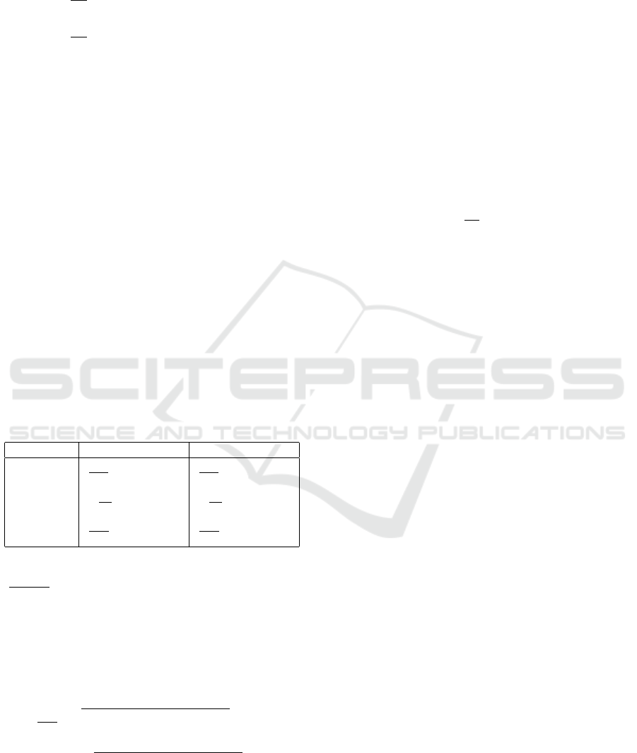
belong to the road. In Fig.2(a,b), we set different val-
ues u and v and a constant K
r
with x
FOE
= y
FOE
= 0.
For the u-component, the image plane is divided into
4 symmetric quarters, each u-value creates a hyper-
bola which is a parallel to each others. Meanwhile for
v-component, the image is divided into 2 symmetric
halfs by the line y
FOE
, each v-value creates a straight
line which is parallel to each other.
2.2 Lateral Plane Model
From the vehicle, buildings can be considered as lat-
eral planes. The principle is the same than for hori-
zontal planes: iso-motion contours of a lateral plane
are shown in Fig.2(c,d).
In this case, iso-motion contours of lateral planes
are symmetric to those that could be computed for
horizontal planes. The iso-motion contours of u-
component forms a straight line parallel to the x
FOE
line.
2.3 Vertical Plane Model
Obstacles could be assimilated to vertical planes in
front of vehicle. As we can see in the Fig.2(e,f), iso-
motion contours of obstacle planes inherit the charac-
teristics of both u component from lateral planes and
v component from horizontal planes.
The straight line of iso-motion curve of v-
component (horizontal plane) or u-component (lateral
plane), that appears is an interesting characteristic that
shows that it is possible to exploit u and v separately
to build dedicated voting spaces.
Exploiting Optical Flow Field Properties for 3D Structure Identification
461

(a) (b) (c) (d) (e) (f)
Figure 2: Iso-motion contours of u-component (a,c,e) and v-component (b,d,f) on the image for horizontal planes (a,b), lateral
plane (c,d) and vertical plane (e,f). The red lines are the axes x (horizontal) and y (vertical). The origin is at their intersection.
3 UV-VELOCITY
In this section, we explain how to create uv-velocity
voting spaces and how to exploit them to detect cor-
responding plane models.
3.1 Voting Spaces
Based on the analysis of iso-motion contours, we pro-
pose to detect three types of planes by using two vot-
ing spaces called u-velocity and v-velocity . Consid-
ering an image of size H ×W , these voting spaces
are respectively of size W ×u
max
and H ×v
max
, where
u
max
and v
max
are the maximum motion values.
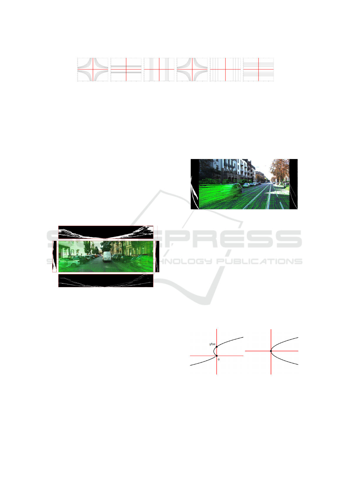
Figure 3: The u-velocity before and after thresholding
(top, bottom respectively) and the v-velocity before and af-
ter thresholding (left, right respectively) represent voting
spaces corresponding to the optical field computed (middle)
for an image sequence from the KITTI dataset.
Each row of the v-velocity space is a velocity his-
togram of the v components for each row in the im-
age. In this space, the iso-motion contours for an hor-
izontal plane form a parabola Fig.3(right) since: v =
K
r
y(y −y
FOE
) = f (y) is a quadratic function which
passes through the origin and y
FOE
. From equations
of Table.1, all pixels that belong to the vertical plane
have the same v. It is the case also for each line but
they form a straight line rather than a parabola Fig.4
(right). Moreover, for lateral planes, v varies with the
change of x. They form arbitrary points with low in-
tensity in the voting space which can be eliminated by
using a threshold Fig.3(left to right, top to bottom),
Fig.3 (left to right). Similarly, the u-velocity space
Fig.3 (bottom) is a set of velocity histogram of the u
components that are constructed by considering each
column of the motion image. The parabolas that ap-
pear on this voting space represent lateral planes. A
straight line appears too if a vertical plane exists on
the scene.
Figure 4: The v-velocity voting space before and after
thresholding (left and right respectively) formed from the
v-component of the image motion (middle). Using an opti-
cal flow ground truth, we can clearly see a parabola and a
nearly straight line in the voting space.
3.2 Analysis and Interpretation
The previous subsection has shown how to construct
suitable voting spaces for detecting each plane ac-
cording to its model (horizontal/lateral/vertical). The
next step consists in detecting lines and parabolas us-
ing a Hough transform, using a common strategy. In
case of a translational motion T = [T
X
,T
Y
,T
Z
], consid-
ering a focus of expansion [x
FOE
,y
FOE
], without loss
of generality, and taking example of v-component of
horizontal plane, we can do the following remarks.
Figure 5: Illustration of one parabola finding on the voting
space. Horizontal axes represent v (a) or |v| (b), with y
FOE
and the origin is not interchangeable or is interchangeable
respectively. The vertical axis represents the pixel’s coordi-
nates.
If we ignore v value sign, the parabola is unique
for each horizontal plane but all parabolas share the
ICINCO 2017 - 14th International Conference on Informatics in Control, Automation and Robotics
462

same vertical-axes coordinates of vertex which is y
v
=
y
FOE
/2 but they have different horizontal-axes coor-
dinates v = K
r
|y
r
|(y
r
−y
FOE
| (see Fig.5(a)). In case
of moving vehicles, the most important translation
in terms of amplitude is toward the Z direction, that
is T
X
≈ 0 and T
Y
≈ 0, it means that x
FOE
≈ 0 and
y
FOE
≈0. So all parabolas share the same vertex point
which is the origin (see Fig.5(b)). Consequently, all
parabolas share the same form v = ay
2
with a an un-
known value. In order to detect parabolas, we propose
a consensus voting process that leads to the estimation
of parameter a.
Finally, the straight lines corresponding to the lat-
eral planes are detected using the Hough transform
after removing pixels that are already labeled as be-
longing to an horizontal or a vertical plane. For point
of extension FOE, knowing that all translation mo-
tions will converge to or diverse from that point. A
voting space where each optical flow draws a straight
line on image are created where the point which has
the most passages is the point of extension. Normally,
this point does not deviate much from the center of
image under our assumption.
4 EXPERIMENTS
To prove the validity of our approach, experiments
are made using first the optical flow ground truth pro-
vided by KITTI and then with the optical flow estima-
tion algorithm proposed by (Sun et al., 2010). For this
first study, only the sequences where translational mo-
tion is dominant are considered. Figures 6 to 8 show a
few examples, where the results of c-velocity and uv-
velocity are put side by side for each kind of plane.
All voting spaces are created using the absolute value
of optical flow for uv-velocity. When using the opti-
cal flow ground truth (top), we got expected results:
planes –especially the horizontal ones (see Fig. 6)–
are correctly detected. Since the optical flow ground
truth is not dense, we focus only on the vehicle and
the road planes (Fig.6,8) since their attributes appear
clearly on the voting space (Fig.4).
By using the optical flow computed from (Sun
et al., 2010) (bottom of figures), the results are not
as good as those we got with ground truth in terms
of precision, occlusion handling (see Fig.6), but the
voting spaces still reveal enough the expected curves
like the one we see in Fig.3. When using the ground
truth, the horizontal plane gives the most reliable re-
sults since it is always available on the image (it cor-
responds to the road). The detection of lateral planes
depends on the scene context, whether it has enough
points to vote for a parabola. Using the Hough trans-
form, the obstacle plane seems to be unstable, since,
for instance, a car always contains many planes. It
means that we have to consider voting space coopera-
tion as future work. However, for some scenes, when
the line appears clearly like in Fig.8, the obstacle can
be detected correctly.
As we can see on Fig.6,7, the uv-velocity give al-
most the same performance as c-velocity whatever the
optical flow, but it avoids expensive calculations like
square-root or exponential and intermediate value c.
5 CONCLUSION
This paper has shown how to detect 3D planes in a
Manhattan world using a specific voting space called
uv-velocity. Its construction is based on the exploita-
tion of optical flow intrinsic properties of moving
planes and more particularly on iso-velocity curves.
Results on ground-truth optical flows prove the effi-
ciency of our new concept, when planes have enough
pixels on the image to be detected. Experiments show
that the precision of the results depends on the the
quality of the input optical flow. In theory, the inter-
ference of other plane models on voting spaces will
not cause much side effects on curve detection be-
cause there contribution in the voting space is low and
could be eliminated by a simple threshold. In practice,
we show that these interferences can complicate line
and parabola detection. One of our futures works is
then to propose a cooperation strategy between voting
spaces. Moreover, since the quality of optical flow is
directly related to the spread of the line or the parabo-
las in the voting space, it is possible to find a met-
ric to find the parabola and refine the optical flow at
the same time (Mai et al., 2017). Finally, rotational
motion will be investigated in next steps to make the
results more general.
REFERENCES
Azuma, T., Sugimoto, S., and Okutomi, M. (2010). Ego-
motion estimation using planar and non-planar con-
straints. In 2010 IEEE Intelligent Vehicles Sympo-
sium, pages 855–862.
Bouchafa, S. and Zavidovique, B. (2012). c-Velocity:
A Flow-Cumulating Uncalibrated Approach for 3d
Plane Detection. International Journal of Computer
Vision, 97(2):148–166.
Cai, Z., Fan, Q., Feris, R. S., and Vasconcelos, N. (2016). A
Unified Multi-scale Deep Convolutional Neural Net-
work for Fast Object Detection. In Computer Vision –
ECCV 2016, pages 354–370. Springer, Cham.
Exploiting Optical Flow Field Properties for 3D Structure Identification
463

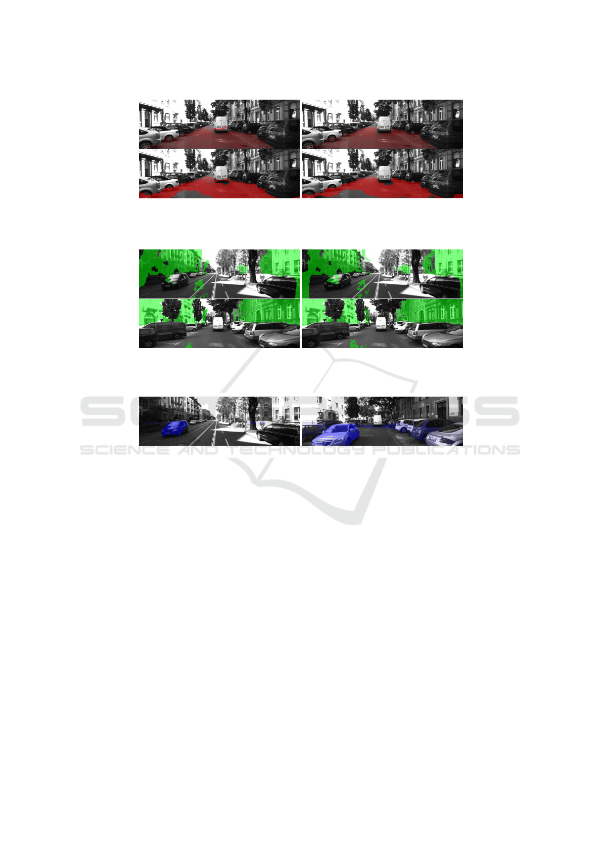
(a) (b)
Figure 6: Horizontal plane detection based on the c-velocity voting space (a) and v-velocity voting space (b) using the optical
flow ground truth (top) and an estimated optical flow (bottom).
(a) (b)
Figure 7: Lateral planes detection whenever they are available on image based on the c-velocity voting space (a) and u-velocity
voting space (b) using the estimated optical flow.
Figure 8: Obstacle detection based on the v-velocity voting space using the optical flow ground truth.
Labayrade, R., Aubert, D., and Tarel, J. P. (2002). Real time
obstacle detection in stereovision on non flat road ge-
ometry through "v-disparity" representation. In IEEE
Intelligent Vehicle Symposium, 2002, volume 2, pages
646–651 vol.2.
Lu, Y., Zhang, J. Z., Wu, Q. M. J., and Li, Z.-N. (2004).
A survey of motion-parallax-based 3-D reconstruc-
tion algorithms. IEEE Transactions on Systems, Man,
and Cybernetics, Part C (Applications and Reviews),
34(4):532–548.
Luong, Q.-T. and Faugeras, O. D. (1997). Camera Calibra-
tion, Scene Motion and Structure recovery from point
correspondences and fundamental matrices. Ijcv,
22:261–289.
Mai, T. K., Gouiffes, M., and Bouchafa, S. (2017). Op-
tical flow refinement using reliable flow propagation.
In Proceedings of the 12th International Joint Con-
ference on Computer Vision, Imaging and Computer
Graphics Theory and Applications - Volume 6: VIS-
APP, (VISIGRAPP 2017), pages 451–458.
Menze, M. and Geiger, A. (2015). Object scene flow for
autonomous vehicles. In Conference on Computer Vi-
sion and Pattern Recognition (CVPR).
Mohan, R. (2014). Deep deconvolutional networks for
scene parsing.
Oliveira, G. L., Burgard, W., and Brox, T. (2016). Efficient
Deep Models for Monocular Road Segmentation.
Qu, L., Wang, K., Chen, L., Gu, Y., and Zhang, X.
(2016). Free Space Estimation on Nonflat Plane
Based on V-Disparity. IEEE Signal Processing Let-
ters, 23(11):1617–1621.
Ren, J., Chen, X., Liu, J., Sun, W., Pang, J., Yan, Q.,
Tai, Y.-W., and Xu, L. (2017). Accurate Single
Stage Detector Using Recurrent Rolling Convolution.
arXiv:1704.05776 [cs]. arXiv: 1704.05776.
Soquet, N., Aubert, D., and Hautiere, N. (2007). Road Seg-
mentation Supervised by an Extended V-Disparity Al-
gorithm for Autonomous Navigation. In 2007 IEEE
Intelligent Vehicles Symposium, pages 160–165.
Sun, D., Roth, S., and Black, M. J. (2010). Secrets of opti-
cal flow estimation and their principles. pages 2432–
2439. IEEE.
ICINCO 2017 - 14th International Conference on Informatics in Control, Automation and Robotics
464