Unscented Kalman Filter for Vision based Target Localisation with a
Quadrotor
Jos Alejandro Dena Ruiz and Nabil Aouf
Centre of Electronic Warfare, Defence Academy of the United Kingdom,
Cranfield University, Shrivenham, SN6 8LA, U.K.
Keywords:
UAV, Unscented Kalman Filter, Optitrack, ROS.
Abstract:
Unmanned aerial vehicles (UAV) equipped with a navigation system and an embedded camera can be used to
estimate the position of a desired target. The relative position of the UAV along with knowledge of camera
orientation and imagery data can be used to produce bearing measurements that allow estimation of target
position. The filter methods applied are prone to biases due to noisy measurements. Further noise may be
encountered depending on the UAV trajectory for target localisation. This work presents the implementation
of an Unscented Kalman Filter (UKF) to estimate the position of a target on the 3D cartesian plane within a
small indoor scenario. A small UAV with a single board computer, equipped with a frontal camera and moving
in an oval trajectory at a fixed height was employed. Such a trajectory enabled an experimental comparison
of UAV simulation data with UAV real-time flight data for indoor conditions. Optitrack Motion system and
the Robot Operative System (ROS) were used to retrieve the drone position and exchange information at high
rates.
1 INTRODUCTION
Unmanned Aerial Vehicles (UAV) have proven to be
a reliable platforms for research. The quadrotor UAV
has been one of the most popular among the different
UAV types, due to the easy architecture and its ca-
pabilities in reaching areas where no other UAV can.
The small size and the vertical take-off and landing
are two of the main advantages this UAV offers.
This paper presents the use of a small quadrotor
with an onboard embedded camera for target localisa-
tion on indoor conditions at low height. Visual mea-
surements of the target based on the pixel position on
the image can be transformed into two bearing mea-
surements, dependent upon the vehicle position and
orientation (Ponda, 2008). The use of bearing angles
based only on the pixel position is not enough to de-
termine the target localisation without the range (and
with noisy measurements), therefore an Unscented
Kalman Filter (UKF) is implemented to estimate a
stationary target position whitin the 3D plane. The
estimation results are influenced by the drone’s trajec-
tory. Therefore an oval trajectory was chosen in order
to vary both measured angles whitin a small area.
Several pieces of research have been done related
to target localisation with UAV, like the use of fixed
wing vehicles with visible cameras on (Hosseinpoor
et al., 2016); (Wang et al., 2016). (Ponda, 2008) pre-
sented the use of an Extended Kalman Filter for target
localisation with a fixed-wing drone and a gimballed
camera, showing simulation results of a localised ob-
ject being orbited by the drone at 100 ft height and
with an orbit of 50 ft radius, achieving the final es-
timated values after 100 measurements. Similarly,
(Redding et al., 2008) used a Recursive Least Squares
(RLS) filter to estimate the target position, achiev-
ing experimental results using a fixed-wing miniature
drone with a circular orbit of 50 m radius and 60 m al-
titude, obtaining an estimation with an error of 10.9 m
after 20 seconds of trajectory. (Deneault et al., 2008)
presented the tracking for ground targets using an Un-
scented Transformation. To obtain the required mea-
surements, mean and covariance data for the target
position as a function of the SLAM states and cam-
era measurements were used. (Hou and Yu, 2014)
show the use of a Pelican quadrotor for target locali-
sation, using a configuration of a frontal camera, ul-
trasonic and laser sensors. The use of these three de-
vices determined the current drone position. An on-
board visible camera was used for object colour de-
tection, experiments shows the target localisation us-
ing this setup. (Jung et al., 2016) presented the use
Ruiz, J. and Aouf, N.
Unscented Kalman Filter for Vision based Target Localisation with a Quadrotor.
DOI: 10.5220/0006474404530458
In Proceedings of the 14th International Conference on Informatics in Control, Automation and Robotics (ICINCO 2017) - Volume 2, pages 453-458
ISBN: Not Available
Copyright © 2017 by SCITEPRESS – Science and Technology Publications, Lda. All rights reserved
453

of an UKF to estimate the position of a moving tar-
get with three different process model. Simulations
on Matlab show different estimation error for each
model where a camera pointing downwards is track-
ing the moving target for landing purposes. (Gomez-
Balderas et al., 2013) used a quadrotor for target lo-
calisation and tracking, controlling the UAV based on
the target localisation to keep it on the field of view,
all under indoor conditions.
2 TECHNICAL APPROACH
A simple projection of the target on the image is pre-
sented in Figure 1. Where the camera pointing axis is
well known, the UAV position is obtained by a motion
capture system and the orientation by the onboard In-
ertial Measurement Unit (IMU). This way the pixel
location can be transformed into two bearing angles
(α
1
and α
2
) from the camera pointing axis to a vec-
tor that passes though the target and the camera focal
point. Using a series of rotations from the camera
frame to the UAV body frame, and from the body
frame to the earth frame, these angles can be con-
verted into overall azimuth and elevation angles (β
and φ), Figure 2, which define the bearing angles be-
tween the UAV and the target.
Figure 1: Image measurement projection based on the target
pixel position.
Figure 2: Azimuth and Elevation β and φ.
3 PLATFORM VEHICLE AND
SCENARIO
A Pelican quadrotor from Ascending Technologies
(AscTec) was chosen as the prototype to develop the
experiments, as its physical architecture made of car-
bon fibre and both well distributed sensors and com-
ponents make it a reliable platform for research pur-
poses. This quadrotor offers plenty of space and var-
ious interfaces for individual components and pay-
loads. Figure 3.
Figure 3: Quadrotor AscTec Pelican used to develop the
experiments.
The basic electronic components are the AscTec Au-
topilot, motor controllers and a single board com-
puter named the Mastermind. The AscTec Autopi-
lot also known as Flight-Control-Unit(FCU), contains
the High Level Processor and the Low Level Proces-
sor (LLP and HLP) running at 1 kHz, which are in
charge of aircraft control. The LLP handles sensor
data processing and data fusion, as well as an stable
attitude control algorithm. The HLP is open for the
user purposes, like the implementation of control al-
gorithms, sensor fusion, etc.
The AscTec Mastermind is an onboard processor
board, its weight of 400 grams and size 10X10X5 cm
offers an extremely high processing power, high data
rates and a great variety of standard PC interfaces.
Features like a Dual Core Atom, a Core 2 Duo, or a
Core i7, WIFI, Firewire and hardware serial ports are
supported. Running Ubuntu 14.04 as operative sys-
tem, the user has plenty of programming possibilities.
The Optitrack Motion Capture System, was used
to retrieve the ground truth position. The full setup
to get the ground truth is composed of six cameras
connected to a 12-port POE switch, along with a host
computer with Optitrack Motive application, that runs
and streams the current position of the rigid body at
120 Hz. The position is published on ROS and re-
trieved by the Mastermind which is also connected to
the same wireless network, Figure 4.
The platform was also equipped with an
mvBlueFox-IGC visible camera, the images are ob-
tained through a ROS package at 20 Hz and published
into the ROS network for its future processing.
ICINCO 2017 - 14th International Conference on Informatics in Control, Automation and Robotics
454

Figure 4: Quadrotor Control System overview.
4 VISION-BASED TARGET
LOCALISATION
This section describes the problem of target locali-
sation using vision-only. The measurements are ob-
tained from the camera on the quadrotor. For the pur-
pose of this project, the image processing for target
recognition is assumed and the pixel location corre-
sponding to the centre of the target is available. This
way, the images from the image sensors can be con-
verted into bearings-only measurements, which can
be processed using the UKF to estimate the location
of the target. Considering that the target is station-
ary, the estimation time and accuracy will be highly
influenced by the drone’s path. In this case an oval
with radius of r1 = 1 m (in the short axis) and radius
r2 = 1.5 m (in the long axis) and a constant height of
0.5 m were chosen in order to vary the measurements
as much as possible in a reduced area.
The target dynamics model is assumed to be linear
but the measurement model is still non-linear, giving
the following system dynamics,
X
k+1
= Φ
k+1,k
X
k
+W
k
(1)
Z
k
= h(X
k
) +V
k
(2)
where Φ
k+1,k
is the state transition matrix of the
system from the time k to k+ 1 and W
k
and V
k
are the
process and measurement noise, which are uncorre-
lated, Gaussian and white with zero mean and covari-
ance Q
k
and R
k
respectively.
Figure 5: Target and vehicle vector representation
The measurement model involves two bearing mea-
surements and is given by
h
x
k
=

β
φ

=
"
tan
−1
(
r
x
r
y
)
tan
−1
(
r
z
√
(r
x
)
2
+(r
y
)
2
)
#
(3)
where r
x
= p
x
−t
x
, r
y
= p
y
−t
y
, r
z
= p
z
−t
z
.
p
k
= [p
x
p
y
p
z
]
T
k
is the quarotor position, t
k
=
[t
x
t
y
t
z
]
T
k
is the target estimated position and r
k
=
[r
x
r
y
r
z
]
T
k
the relative vector between the vehicle
and the target respectively, Figure 5.
5 UNSCENTED KALMAN FILTER
The UKF algorithm is composed by the time up-
date and measurement update steps. The time up-
date includes the weights and sigma points calcu-
lations, whereas the measurement update uses the
sigma points to generate the covariance matrices and
the kalman gain respectively.
5.1 Time Update
First, weights are defined as:
W
1
=
λ
n+ λ
(4)
W
i
=
1
2(n+ λ)
i = 1, 2, ...n (5)
where n is the dimension of the state vector and λ
is an arbitrary constant. The sigma points at time step
k calculate as:
S
k−1
= chol((n+ λ)P
k−1
) (6)
X
(0)
= ˆx
k−1
(7)
X
(i)
= ˆx
k−1
+ S
(i)
k−1
i = 1, 2, ...n (8)
X
(i+n)
= ˆx
k−1
−S
(i)
k−1
i = 1, 2, ...n (9)
X
k−1
= [X
(0)
X
(1)
···X
(2n)
] (10)
chol means cholesky decomposition and S
(i)
mean
ith row vector of S. The time update equations are:
ˆ
X
k
=
2n
∑
i=0
W
i
f(X
i
) (11)
P
k
=
2n
∑
i=0
W
i
{f(X
i
) −
ˆ
X
k
}{f(X
i
) −
ˆ
X
k
}
T
+ Q
k
(12)
Unscented Kalman Filter for Vision based Target Localisation with a Quadrotor
455

5.2 Measurement Update
The augmented sigma points are calculated as fol-
lows:
S
k
= chol((n + λ)P
k
) (13)
X
(0)
= ˆx
k
(14)
X
(i)
= ˆx
k
+ S
(i)
k
i = 1, 2, ...n (15)
X
(i+n)
= ˆx
k
−S
(i)
k
i = 1, 2, ...n (16)
X
k
= [X
(0)
X
(1)
···X
(2n)
] (17)
ˆz
k
=
2n
∑
i=0
W
i
h(X
i
) (18)
The measurement update equations are:
P
z
=
2n
∑
i=0
W
i
{h(X
i
) − ˆz
k
}{h(X
i
) − ˆz
k
}
T
+ R(19)
P
xz
=
2n
∑
i=0
W
i
{f(X
i
) − ˆx
k
}{h(X
i
) − ˆz
k
}
T
(20)
The Kalman gain is calculated as:
K
k
= P
xz
P
−1
z
(21)
Finally, the estimated states and it’s covariance
matrix are:
ˆ
X
k
=
ˆ
X
k
+ K
k
(z
k
−ˆz
k
) (22)
P
k
= P
k
−K
k
P
z
K
T
k
(23)
For this scenario with an stationary target, the pro-
cess noise is zero because the target position is con-
stant. The process model, process error covariance
matrix and the measurement covariance error are:
Φ
k,k−1
=


1 0 0
0 1 0
0 0 1


, Q
k
=


0 0 0
0 0 0
0 0 0


(24)
R
k
=

σ
2
1
0
0 σ
2
2

(25)
6 SIMULATION AND
EXPERIMENTAL RESULTS
The target estimation algorithm for simulations and
experiments was initialised with the following param-
eters,
ˆ
X
0
=


20
20
20


, P
0
=


50 0 0
0 50 0
0 0 50


, λ = 0 (26)
in both cases, the quadrotor trajectory is running
at 15Hz (step k=0.066 sec) and 0.01 radians per step.
At every step the camera takes an image which is pro-
cessed to locate the target. Once the pixel that repre-
sents the centre of the target is obtained this pixel is
mapped into the bearing angles, which will be taken
by the UKF along with the drone position and orien-
tation, to estimate the 3D target position.
6.1 Simulation
Gazebo Simulator and ROS were used as the virtual
environment to simulate the estimation, the package
rotors simulator (Furrer et al., 2016) provides some
multi-rotor models such as the AscTec Hummingbird,
the AscTec Pelican, or the AscTec Firefly. In the
package files, the user can select the model to work
with as well as plenty of sensors. The Pelican quadro-
tor and a visible camera were selected. An small black
cylinder was used as a target for simulations(Figure
6), positioned on the 3D plane coordinates 2.85, 0.05
and 0.0 (x, y, z respectively). For this simulation, the
noise that affects the measurement is coming from the
camera. White gaussian noise with zero mean noise
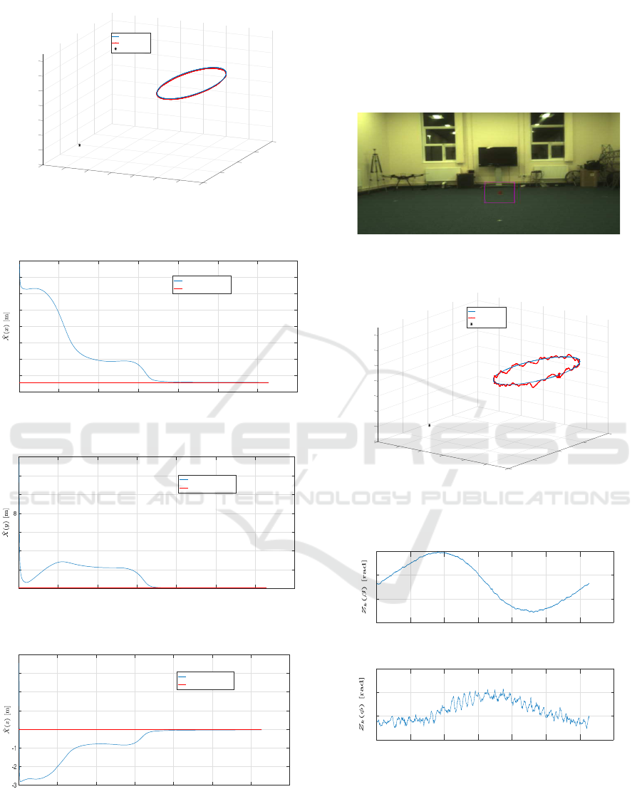
was added with standard deviation σ = 0.007. Fig-
ure 7 shows the target position and UAV trajectory,
whereas Figures 9-11 show the estimated results for
each axis.
Figure 6: Image retrieved from the virtual image sensor
pointing at the target.
6.2 Experiments
The experiments were performed in indoor condi-
tions. To control the Pelican quadrotor position,
Optitrack Motion Capture was used to feedback the
ground truth, which is published by ROS at 120 Hz.
As a target on the real UAV flight experiments a red
cup was used for simplicity, positioned in the same
coordinates as on simulations(Figure 11). The im-
age sensor used for the experiment was the BlueFox
IGC202C, publishing images at 20 Hz on ROS. The
ICINCO 2017 - 14th International Conference on Informatics in Control, Automation and Robotics
456

-2
-1
Y position in metres
Oval trajectory for target localisation
0
0
0.1
3
0.2
2
0.3
1
1
X position in metres
Z position in metres
0.4
0
0.5
-1
0.6
-2
0.7
-3
2
-4
Desired trajectory
Drone trajectory
Target
Figure 7: 3D view of the flight path on simulations and tar-
get position.
0 100 200 300 400 500 600 700
Number of Measurements [k]
0
5
10
15
20
25
30
35
40
X Position Estimation
Estimated position
Real position
Figure 8: Estimation of
ˆ
X(x) on simulation.
0 100 200 300 400 500 600 700
Number of Measurements [k]
0
2
4
6
10
12
14
Y Position Estimation
Estimated position
Real position
Figure 9: Estimation of
ˆ
X(y) on simulation.
0 100 200 300 400 500 600 700
Number of Measurements [k]
0
1
2
3
4
Z Position Estimation
Estimated position
Real position
Figure 10: Estimation of
ˆ
X(z) on simulation.
use of gimbal was not necessary, because the target
never left the camera field of view. The noise on
the measurement is coming from the image sensor.
Several tests with the target and Drone being station-
ary were made in order to get the variance of this
noise, σ
2
1
= 4.65X10
−5
and σ
2
2
= 6.5X10
−8
. Figure
12 shows the target position and UAV trajectory, Fig-
ure 13 shows the noisy measurements and Figures 14-
16 show the estimated results for each axis.
Figure 11: Image retrieved from the image sensor on exper-
iments.
-2
0
0.1
-1
3
0.2
Oval trajectory for target localisation
0.3
2
0.4
Z position in metres
Y position in metres
0
0.5
1
0.6
X position in metres
0
0.7
1
-1
-2
2
-3
Desired trajectory
Drone trajectory
Target
Figure 12: 3D view of the flight path on experiments and
target position.
0 100 200 300 400 500 600 700
Number of Measurements [k]
2.8
3
3.2
3.4
Measured Azimut Angle
0 100 200 300 400 500 600 700
Number of Measurements [k]
0.05
0.1
0.15
0.2
Measured Elevation Angle
Figure 13: Measurements(Z
k
), Azimut (β) and Elevation (φ)
angles based on the pixel position.
Unscented Kalman Filter for Vision based Target Localisation with a Quadrotor
457

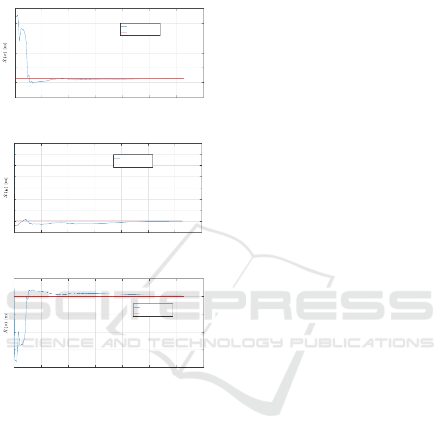
0 100 200 300 400 500 600 700
Number of Measurements [k]
-10
0
10
20
30
40
50
X Position Estimation
Estimated position
Real position
Figure 14: Estimation of
ˆ
X(x) on experiment.
0 100 200 300 400 500 600 700
Number of Measurements [k]
-2
0
2
4
6
8
10
12
14
Y Position Estimation
Estimated position
Real position
Figure 15: Estimation of
ˆ
X(y) on experiment.
0 100 200 300 400 500 600 700
Number of Measurements [k]
-4
-3
-2
-1
0
1
Z Position Estimation
Estimated position
Real position
Figure 16: Estimation of
ˆ
X
(z)
on experiment.
7 CONCLUSIONS
This paper shows the implementation of an UKF for
target localisation with simulations and experimental
results using bearing angles only. The quadrotor uses
a frontal camera that captures the target on the im-
age. The image is processed in order to obtain the
pixel that represents the target centre, which along
with the drone position and orientation, can be con-
verted into the azimuth and elevation. The UKF was
fed with the noisy azimuth and elevation angles and
estimates the 3D target position. The simulation re-
sults show that the estimated values converged into
the real values after 400 measurements on the 3 axis,
whereas in the experimental results the estimated val-
ues converged in 500 measurements. On real and sim-
ulation results, the
ˆ
X(z) axis presents the bigger error
in steady state 0.07 m and 0.035 m, due to the lack
of the vector range between the drone and the target.
The final errors for
ˆ
X(x) and
ˆ
X(y) on simulation were
0.07 m and 0.028 m, as opposed to 0.018 m and 0.05
m for experimental results. The simulation was ran
under Gazebo Simulator and ROS, whereas for UAV
real-time flight experiments Optitrack and ROS were
used to perform the full estimation algorithm. The
complete set-up allowed us to perform the estimation
in real-time, and achieving the target position after 30
seconds of trajectory. The use of additional, differ-
ent trajectories would reduce the estimation time like
showed (Ponda, 2008), although for indoor environ-
ments with a reduced area, the presented trajectory
and estimator performed successfully.
REFERENCES
Deneault, D., Schinstock, D., and Lewis, C. (2008). Track-
ing ground targets with measurements obtained from
a single monocular camera mounted on an unmanned
aerial vehicle. Proceedings - IEEE International Con-
ference on Robotics and Automation, pages 65–72.
Furrer, F., Burri, M., Achtelik, M., and Siegwart, R. (2016).
RotorSA modular gazebo MAV simulator framework.
Studies in Computational Intelligence, 625:595–625.
Gomez-Balderas, J. E., Flores, G., Garc´ıa Carrillo, L. R.,
and Lozano, R. (2013). Tracking a Ground Mov-
ing Target with a Quadrotor Using Switching Control.
Journal of Intelligent & Robotic Systems, 70(1-4):65–
78.
Hosseinpoor, H. R., Samadzadegan, F., and Dadrasjavan,
F. (2016). Pricise Target Geolocation and Tracking
Based on Uav Video Imagery. In ISPRS - Interna-
tional Archives of the Photogrammetry, Remote Sens-
ing and Spatial Information Sciences, volume XLI-
B6, pages 243–249.
Hou, Y. and Yu, C. (2014). Autonomous target localization
using quadrotor. 26th Chinese Control and Decision
Conference, CCDC 2014, pages 864–869.
Jung, W., Kim, Y., and Bang, H. (2016). Target state esti-
mation for vision-based landing on a moving ground
target. 2016 International Conference on Unmanned
Aircraft Systems, ICUAS 2016, pages 657–663.
Ponda, S. (2008). Trajectory Optimization for Target Local-
ization Using Small Unmanned Aerial Vehicles. AIAA
Guidance, Navigation, and Control Conference, (Au-
gust).
Redding, J., McLain, T., Beard, R., and Taylor, C. (2008).
Vision-based Target Localization from a Fixed-wing
Miniature Air Vehicle. 2006 American Control Con-
ference, 44(4):2862–2867.
Wang, X., Liu, J., and Zhou, Q. (2016). Real-time multi-
target localization from Unmanned Aerial Vehicle.
Sensors, pages 1–19.
ICINCO 2017 - 14th International Conference on Informatics in Control, Automation and Robotics
458