Demand Prediction using Machine Learning Methods and Stacked

Generalization

Resul Tugay and S¸ule G

und

Og¸

Department of Computer Engineering, Istanbul Technical University, Istanbul, Turkey

Keywords:

Stacked Generalization, Random Forest, Demand Prediction.

Abstract:

Supply and demand are two fundamental concepts of sellers and customers. Predicting demand accurately

is critical for organizations in order to be able to make plans. In this paper, we propose a new approach for

demand prediction on an e-commerce web site. The proposed model differs from earlier models in several

ways. The business model used in the e-commerce web site, for which the model is implemented, includes

many sellers that sell the same product at the same time at different prices where the company operates a

market place model. The demand prediction for such a model should consider the price of the same product

sold by competing sellers along the features of these sellers. In this study we ﬁrst applied different regression

algorithms for speciﬁc set of products of one department of a company that is one of the most popular online

e-commerce companies in Turkey. Then we used stacked generalization or also known as stacking ensemble

learning to predict demand. Finally, all the approaches are evaluated on a real world data set obtained from the

e-commerce company. The experimental results show that some of the machine learning methods do produce

almost as good results as the stacked generalization method.

1 INTRODUCTION

Demand forecasting is the concept of predicting the

quantity of a product that consumers will purchase

during a speciﬁc time period. Predicting right demand

of a product is an important phenomenon in terms of

space, time and money for the sellers. Sellers may

have limited time or need to sell their products as soon

as possible due to the storage and money restrictions.

Therefore demand of a product depends on many fac-

tors such as price, popularity, time, space etc. Fore-

casting demand is being hard when the number of fac-

tors increases. Demand prediction is also closely re-

lated with seller revenue. If sellers store much more

product than the demand then this may lead to sur-

plus (Miller et al., 1988). On the other hand storing

less product in order to save inventory costs when the

product has high demand will cause less revenue. Be-

cause of these and many more reasons, demand fore-

casting has become an interesting and important topic

for researchers in many areas such as water demand

prediction (An et al., 1996), data center application

(Gmach et al., 2007) and energy demand prediction

(Srinivasan, 2008).

The rest of the paper is organized as fol-

lows:Section 2 discusses related work and section 3

describe methodology. In section 5 we describe our

experimental results and data deﬁnitions. In section 6

we conclude this work and future work.

2 RELATED WORK

In literature, the research studies on demand forecast-

ing can be grouped into three main categories: (1) Sta-

tistical Methods; (2) Artiﬁcial Intelligence Methods;

(3) Htybrid Methods.

Statistical Methods. Linear regression, regression

tree, moving average, weighted average, bayesian

analysis are just some of statistical methods for de-

mand forecasting (Liu et al., 2013). Johnson et al.

used regression trees to predict demand due to its

simplicity and interpretability (Johnson et al., 2014).

They applied demand prediction on data given by an

online retailer web company named as Rue La La.

The web site consists of several events which are

changing within 1-4 days interval from different de-

partments. Each event has multiple products called

”style” and each product has different items. Items

are typical products that have different properties such

as size and color. Because of the price is set at style

level, they aggregate items at style level and use dif-

216

Tugay, R. and Ö

güdücü, ¸S.

Demand Prediction using Machine Learning Methods and Stacked Generalization.

DOI: 10.5220/0006431602160222

In Proceedings of the 6th International Conference on Data Science, Technology and Applications (DATA 2017), pages 216-222

ISBN: 978-989-758-255-4

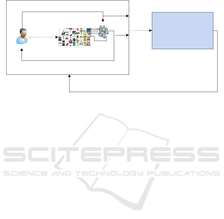
Customer

orders a product

Web Site

Sellers

Shipping ß N

Seller

Reviews product Quality/

shipping/Seller Reponse

etc.

Training Data

STACKED GENERALIZATION SYSTEM

WebSite ß Demand Prediction

Figure 1: General System Schema.

ferent regression models for each department. Edi-

ger and Akar used Autoregressive Integrated Moving

Average (ARIMA) and seasonal ARIMA (SARIMA)

methods to predict future energy demand of Turkey

from 2005 to 2020 (Ediger and Akar, 2007). Also Lim

and McAleer used ARIMA for travel demand fore-

casting (Lim and McAleer, 2002).

Although basic implementation and simple interpre-

tation of statistical methods, different approaches are

applied for demand forecasting such as Artiﬁcial In-

telligence (AI) and hybrid methods.

AI Methods. AI methods are commonly used in lit-

erature for demand forecasting due to their primary

advantage of being efﬁcient and accurate (Chang and

Wang, 2006), (Gutierrez et al., 2008), (Zhang et al.,

1998), (Yoo and Pimmel, 1999). Frank et al. used Ar-

tiﬁcial Neural Networks (ANN) to predict women’s

apparel sales and ANN outperformed two statistical

based models (Frank et al., 2003). Sun et al. proposed

a novel extreme learning machine which is a type of

neural network for sales forecasting. The proposed

methods outperformed traditional neural networks for

sales forecasting (Sun et al., 2008).

Hybrid Methods. Another method of forecasting

sales or demands is hybrid methods. Hybrid methods

utilize more than one method and use the strength of

these methods. Zhang used ARIMA and ANN hybrid

methodology in time series forecasting and proposed

a method that achieved more accuracy than the meth-

ods when they were used separately (Zhang, 2003). In

addition to hybrid models, there has been some stud-

ies where fuzzy logic is used for demand forecasting

(Aburto and Weber, 2007), (Thomassey et al., 2002),

(Vroman et al., 1998).

Thus far, many researchers focused on different

statistical, AI and hybrid methods for forecasting

problem. But Islek and Gunduz Oguducu proposed

a state-of-art method that is based on stack gener-

alization on the problem of forecasting demand of

warehouses and their model decreased the error rate

using proposed method (Islek, 2016). On the con-

trary, in this paper we use different statistical meth-

ods and compare their results with stack generaliza-

tion method which uses these methods as sub-level

learners.

3 METHODOLOGY

This section describes the methodology and tech-

niques used to solve demand prediction problem.

3.1 Stacked Generalization

Stacked generalization (SG) is one of the ensemble

methods applied in machine learning which use multi-

ple learning algorithms to improve the predictive per-

formance. It is based on training a learning algorithm

to combine the predictions of the learning algorithms

involved instead of selecting a single learning algo-

rithm. Although there are many different ways to

implement stacked generalization, its primary imple-

mentation consists of two stages. At the ﬁrst stage, all

the learning algorithms are trained using the available

data. At this stage, we use linear regression, random

forest regression, gradient boosting and decision tree

regression as the ﬁrst-level regressors. At the second

stage a combiner algorithm is used to make a ﬁnal

prediction based on all the predictions of the learning

algorithms applied in the ﬁrst stage. At this stage, we

Demand Prediction using Machine Learning Methods and Stacked Generalization

217

use again same regression algorithms we used in the

ﬁrst stage to specify which model is the best regressor

for this problem. The general schema of stacked gen-

eralization applied in this study can be seen in Figure

Gradient Boosted

Trees

Linear Regression

Training

Data

Random Forest

Meta-Regressor

Prediction

Last

Prediction

Decision Tree

Prediction

Figure 2: Stacked Generalization.

3.2 Linear Regression

A linear regression (LR) is a statistical method where

a dependent variable γ (the target variable) is com-

puted from p independent variables that are assumed

to have an inﬂuence on the target variable. Given a

data set of n data points, the formula for a regression

of one data point γ

(regressand) is as follows:

= β

+ ..β

+ ε

i = 1, 2, ..n (1)

where β

is the regression coefﬁcient that can be cal-

culated using Least Squares approach, x

i j

(regressor)

is the value of the j

independent variable and ε

the

error term. The best-ﬁtting straight line for the ob-

served data is calculated by minimizing the loss func-

tion which is sum of the squares of differences be-

tween the value of the point γ

and the predicted value

(the value on the line) as shown in Equation 2.

MSE =

∑

i=1

(

− γ

)

(2)

The best values of regression coefﬁcients and the er-

ror terms can be found by minimizing the loss func-

tion in Equation 2. While minimizing loss function,

a penalty term is used to control the complexity of

the model. For instance, lasso (least absolute shrink-

age and selection operator) uses L1 norm penalty term

and ridge regression uses L2 norm penalty term as

shown in Equation (3) and (4) respectively. λ is reg-

ularization parameter that prevents overﬁtting or con-

trols model complexity. In both Equation (3) and (4)

coefﬁcients (β), dependent variables (γ) and indepen-

dent variables (X) are represented in matrix form.

β = argmin{

(γ − βX)

+ λ

||β||

} (3)

β = argmin{

(γ − βX)

+ λ

||β||

} (4)

In this study, we used elastic net which is combina-

tion of L1 and L2 penalty terms with λ = 0.8 for L1

and λ = 0.2 for L2 penalty term with λ = 0.3 regular-

ization parameter as shown in Equation (5).

β = argmin{

(γ − βX)

+ λ(0.8||β||

+ 0.2||β||

)}

(5)

3.3 Decision Tree Regression

Decision trees (DT) can be used both in classiﬁcation

and regression problems. Quinlan proposed ID3 al-

gorithm as the ﬁrst decision tree algorithm (Quinlan,

1986). Decision tree algorithms classify both categor-

ical (classiﬁcation) and numerical (regression) sam-

ples in a form of tree structure with a root node, in-

ternal nodes and leaf nodes. Internal nodes contain

one of the possible input variables (features) avail-

able at that point in the tree. The selection of input

variable is chosen using information gain or impurity

for classiﬁcation problems and standard deviation re-

duction for regression problems. The leaves repre-

sent labels/predictions. Random forest and gradient

boosting algorithms are both decision tree based al-

gorithms. In this study, decision tree method is ap-

plied for regression problems where variance reduc-

tion is employed for selection of variables in the inter-

nal nodes. Firstly, variance of root node is calculated

using Equation 6, then variance of features is calcu-

lated using Equation 7 to construct the tree.

∑

i=1

− µ)

(6)

In Equation 6, n is the total number of samples and

µ is the mean of the samples in the training set. Af-

ter calculating variance of the root node, variance of

input variables is calculated as follows:

∑

cεX

P(c)σ

(7)

In Equation 7, X is the input variable and c’s are the

distinct values of this feature. For example, X : Brand

and c : Samsung, Apple or Nokia. P(c) is the proba-

bility of c being in the attribute X and σ

is the vari-

ance of the value c. Input variable that has the mini-

mum variance or largest variance reduction is selected

as the best node as shown in Equation 8:

= σ

− σ

(8)

Finally leaves are representing the average values of

instances that they include in subsection 3.4 with

DATA 2017 - 6th International Conference on Data Science, Technology and Applications

218

bootstrapping method. This process continues recur-

sively, until variance of leaves is smaller than a thresh-

old or all input variables are used. Once a tree has

been constructed, new instance is tested by asking

questions to the nodes in the tree. When reaching a

leaf, value of that leaf is taken as prediction.

3.4 Random Forest

Random forest (RF) is a type of meta learner that uses

number of decision trees for both classiﬁcation and

regression problems (Breiman, 2001). The features

and samples are drawn randomly for every tree in the

forest and these trees are trained independently. Each

tree is constructed with bootstrap sampling method.

Bootstrapping relies on sampling with replacement.

Given a dataset D with N samples, a training data set

of size N is created by sampling from D with replace-

ment. The remaining samples in D that are not in the

training set are separated as the test set. This kind of

sampling is called bootstrap sampling.

The probability of an example not being chosen in

the dataset that has N samples is :

Pr = 1 −

(9)

The probability of being in the test set for a sample is:

Pr =



1 −



≈ exp

−1

= 0.368 (10)

Every tree has a different test set and this set consists

of totally %63.2 of data. Samples in the test set are

called out-of-bag data. On the other hand, every tree

has different features which are selected randomly.

While selecting nodes in the tree, only a subset of the

features are selected and the best one is chosen as sep-

arator node from this subset. Then this process con-

tinues recursively until a certain error rate is reached.

Each tree is grown independently to reach the speci-

ﬁed error rate. For instance, stock feature is chosen

as the best separator node among the other randomly

selected features, and likewise price feature is chosen

as second best node for the ﬁrst tree in Figure 3. This

tree is constructed with two nodes such as stock and

price, whereas TREE N has four nodes and some of

them are different than the TREE 1.

Due to bootstrapping sampling method, there is no

need to use cross-validation or separate datasets for

training and testing. This process is done internally.

In this project, minimum root mean squared error was

achieved by using random forest with 20 trees in the

ﬁrst level.

STOCK < 50

YES

100 50

PRICE < 500

YES

SELLER GRADE > 85

YES

PRICE < 750

YES

TREE 1

TREE N

7020

STOCKOUT

YES

150

FASTSHIP

YES

Figure 3: Random Forest.

3.5 Gradient Boosted Trees

Gradient Boosted Trees (GBT) are ensemble learn-

ing of decision trees (Friedman, 2001). GBT are said

to be the combination of gradient descent and boost-

ing algorithms. Boosting methods aim at improv-

ing the performance of classiﬁcation task by convert-

ing weak learners to strong ones. There are multi-

ple boosting algorithms in literature (Oza and Rus-

sell, 2001), (Grabner and Bischof, 2006), (Grabner

et al., 2006), (Tutz and Binder, 2006). Adaboost is

the ﬁrst boosting algorithm proposed by Freund and

Schapire (Freund et al., 1999). It works by weight-

ing each sample in the dataset. Initially all samples

are weighted equally likely and after each training it-

eration, misclassiﬁed samples are re-weighted more

heavily. Boosting algorithms consist of many weak

learners and use weighted summation of them. A

weak learner can be deﬁned as a learner that performs

better than random guessing and it is used to compen-

sate the shortcomings of existing weak learners. Gra-

dient boosted trees uses gradient descent algorithm

for the shortcomings of weak learners instead of us-

ing re-weighting mechanism. This algorithm is used

to minimize the loss function (also called error func-

tion) by moving in the opposite direction of the gra-

dient and ﬁnds a local minimum. In literature, there

are several different loss functions such as Gaussian

, Laplace L

, Binomial Loss functions etc (Natekin

and Knoll, 2013). Squared-error loss function, com-

monly used in many regression problems, is used in

this project.

Let L(y

, F(x

)) be the loss function where y

is ac-

tual output and F(x

) is the model we want to ﬁt in.

Our aim is to minimize J =

∑

i=1

− F(x

))

func-

tion.By using gradient descent algorithm,

F(x

) = F(x

) − α

δJ

δF(x

)

(11)

In Equation 11, α is learning rate that accelerates

Demand Prediction using Machine Learning Methods and Stacked Generalization

219

or decelerates the learning process. If the learning

rate is very large then optimal or minimal point may

be skipped. If the learning rate is too small, more iter-

ations are required to ﬁnd the minimum value of the

loss function. While trees are constructed in parallel

or independently in random forest ensemble learning,

they are constructed sequential in gradient boosting.

Once all trees have been trained, they are combined

to give the ﬁnal output.

4 EXPERIMENTAL RESULTS

4.1 Dataset Deﬁnition

The data used in the experiments was provided from

one of the most popular online e-commerce company

in {Country Name}. First, standard preprocessing

techniques are applied. Some of these techniques in-

clude ﬁlling in the missing values, removal of missing

attributes when a major portion of the attribute val-

ues are missing and removal of irrelevant attributes.

Each product/good has a timestamp which represents

the date it is sold consisting of year, month, week

and day information. A product can be sold several

times within the same day from both same and dif-

ferent sellers. The demands or sales of a product are

aggregated weekly. While the dataset contains 3575

instances and 17 attributes, only 1925 instances re-

mained after the aggregation. Additionally, customers

enter the company’s website and choose a product

they want. When they buy that product, this operation

is inserted into a table as an instance, but if they give

up to buy, this operation is also inserted into another

table. We used this information to ﬁnd the popular-

ity of the product/good. For instance, product A is

viewed 100 times and product B is viewed 55 times

from both same and different users. It can be con-

cluded that product A is more popular than product B.

Before applying stacked generalization method, out-

liers were removed, we only consider the products

where demand is less than 20. In this study, the pa-

rameters at the data preparation stages are determined

by consulting with our contacts at the e-commerce

company.

4.2 Evaluation Method

We used Root Mean Squared Error (RMSE) to evalu-

ate model performances. It is square root of the sum-

mation of differences between actual and predicted

values. RMSE is frequently used in regression anal-

ysis. RMSE can be calculated as shown in Equation

12.

’s are predicted and γ’s are actual values.

RMSE =

∑

i=1

(

− γ)

(12)

We compared the results of the SG method with

the results obtained by single classiﬁers. These clas-

siﬁers include DT, GBT, RF and LR. Firstly, we split

the data into training, validation and test sets (use %50

of data for training, %20 of data for validation and

the remaining part for testing) and trained ﬁrst level

regressors using the training set. For SG, we applied

10-fold cross validation on the training set to get the

best model of the ﬁrst level regressors (except random

forest ensemble model). After getting the ﬁrst level

regressor models, we used the validation set to create

second level of the SG model. The single classiﬁers

are trained on the combined training and test sets. The

results of single classiﬁers and SG are evaluated us-

ing the test set in terms of RMSE. This process can be

seen in Figure 4.

4.3 Result and Discussion

In this section, we evaluate the proposed model using

RMSE evaluation method. After calculating RMSE

for single classiﬁers and SG, we applied analysis of

variances (ANOVA) test. It is generalized version of

t-test to determine whether there are any statistically

signiﬁcant differences between the means of two or

more unrelated groups. We use ANOVA test to show

that predictions of the models are statistically differ-

ent. The training set is divided randomly into 20 dif-

ferent subsets, so that no subset contains the whole

training set. Using each of the different subsets and

the validation set, the SG model is trained and eval-

uated on the test set. In the ﬁrst level of the SG

model, various combinations of the four algorithms

are used. We also conducted experiments with differ-

ent machine learning algorithms in the second level

of SG. For the single classiﬁers, the combination of

training and tests is divided randomly into 20 subsets,

and the same evaluation process is also repeated for

DATASET

TRAINING SET (%50)

VALIDATION

SET (%20)

RANDOM FOREST

GRADIENT BOOSTED

DECISION TREE

LINEAR REGRESSION

Level

LINEAR REGRESSION

DECISION TREE

GRADIENT BOOSTED

RANDOM FOREST

TEST SET

(%30)

Level

Figure 4: Stacking Process.

DATA 2017 - 6th International Conference on Data Science, Technology and Applications

220

Table 1: The Results of

Regressors at Level 2.

Model RMSE

DT 2.200

GBT 2.299

RF 2.120

LR 1.910

Table 2: The Best Results of

Single Classiﬁers and SG.

Model RMSE

DT 1.928

GBT 1.918

RF 1.865

LR 2.708

SG(LR) 1.864

Table 3: SG with Binary

Combination of Regressors.

Model RMSE

GBT+DT 1,955

GBT+LR 1,957

LR+DT 1,962

DT+RF 1,963

GBT+RF 1,870

LR+RF 1,927

Table 4: SG with Triple Com-

bination of Regressors.

Model RMSE

DT+RF+GBT 1.894

RF+DT+LR 1.909

GBT+LR+DT 2.011

LR+RF+GBT 1.864

these classiﬁers. We also run the proposed method

with different combinations of the ﬁrst level regres-

sors.

Table 1 shows the the average of the RMSE re-

sults of the SG when using different learning methods

in the second level. As can be seen from the table,

LR outperforms the other learning methods. For this

reason, in the remaining experiments, the results of

the SG model is given when using LR in the second

level. Table 2 shows the best results of single classi-

ﬁers and SG model obtained from 20 runs. The SG

model gives the best result when LR, RF and GBT

are used in the ﬁrst level. Table 3 shows the results

of binary combinations of the models. We found the

minimum RMSE as 1.870 by using GBT and RF to-

gether in the ﬁrst level. After using binary combina-

tion of the models in the ﬁrst level, we also created

triple combination of them to specify the best combi-

nation. Table 4 shows results of triple combination of

models.

In ANOVA test, the null hypothesis rejected with

5% signiﬁcance level which shows that the predic-

tions of RF and LR are signiﬁcantly better than others

in the ﬁrst and second level respectively.

After concluding RF and LR are statistically dif-

ferent than other regressors at level 1 and 2 respec-

tively, we applied t-test again with α = 0.05 between

RF in the ﬁrst level and LR in the second level. Result

of the t-test showed that LR in the second level is not

statistically signiﬁcantly different than RF

5 CONCLUSION AND FUTURE

WORK

In this paper, we examine the problem of demand

forecasting on an e-commerce web site. We proposed

stacked generalization method consists of sub-level

regressors. We have also tested results of single clas-

siﬁers separately together with the general model. Ex-

periments have shown that our approach predicts de-

mand at least as good as single classiﬁers do, even

better using much less training data (only %20 of

the dataset). We think that our approach will predict

much better than other single classiﬁers when more

data is used. Because of the difference is not statisti-

cally signiﬁcant between the proposed model and ran-

dom forest, the proposed method can be used to fore-

cast demand due to its accuracy with less data. In the

future, we will use the output of this project as part of

price optimization problem which we are planning to

work on.

ACKNOWLEDGEMENTS

The data used in this study was provided by n11

(www.n11.com). The authors are also thankful for the

assistance rendered by

Ilker K

uc¸

ukil in the production

of the data set.

REFERENCES

Aburto, L. and Weber, R. (2007). Improved supply chain

management based on hybrid demand forecasts. Ap-

plied Soft Computing, 7(1):136–144.

An, A., Shan, N., Chan, C., Cercone, N., and Ziarko, W.

(1996). Discovering rules for water demand predic-

tion: an enhanced rough-set approach. Engineering

Applications of Artiﬁcial Intelligence, 9(6):645–653.

Breiman, L. (2001). Random forests. Machine learning,

45(1):5–32.

Chang, P.-C. and Wang, Y.-W. (2006). Fuzzy delphi

and back-propagation model for sales forecasting

in pcb industry. Expert systems with applications,

30(4):715–726.

Ediger, V. S¸ . and Akar, S. (2007). Arima forecasting of pri-

mary energy demand by fuel in turkey. Energy Policy,

35(3):1701–1708.

Frank, C., Garg, A., Sztandera, L., and Raheja, A. (2003).

Forecasting women’s apparel sales using mathemati-

cal modeling. International Journal of Clothing Sci-

ence and Technology, 15(2):107–125.

Freund, Y., Schapire, R., and Abe, N. (1999). A short in-

troduction to boosting. Journal-Japanese Society For

Artiﬁcial Intelligence, 14(771-780):1612.

Friedman, J. H. (2001). Greedy function approximation: a

gradient boosting machine. Annals of statistics, pages

1189–1232.

Demand Prediction using Machine Learning Methods and Stacked Generalization

221

Gmach, D., Rolia, J., Cherkasova, L., and Kemper, A.

(2007). Workload analysis and demand prediction of

enterprise data center applications. In 2007 IEEE 10th

International Symposium on Workload Characteriza-

tion, pages 171–180. IEEE.

Grabner, H. and Bischof, H. (2006). On-line boosting

and vision. In Computer Vision and Pattern Recog-

nition, 2006 IEEE Computer Society Conference on,

volume 1, pages 260–267. IEEE.

Grabner, H., Grabner, M., and Bischof, H. (2006). Real-

time tracking via on-line boosting. In Bmvc, volume 1,

page 6.

Gutierrez, R. S., Solis, A. O., and Mukhopadhyay, S.

(2008). Lumpy demand forecasting using neural net-

works. International Journal of Production Eco-

nomics, 111(2):409–420.

Islek, I. (2016). Using ensembles of classiﬁers for demand

forecasting.

Johnson, K., Lee, B. H. A., and Simchi-Levi, D. (2014).

Analytics for an online retailer: Demand forecasting

and price optimization. Technical report, Technical

report). Cambridge, MA: MIT.

Lim, C. and McAleer, M. (2002). Time series forecasts

of international travel demand for australia. Tourism

management, 23(4):389–396.

Liu, N., Ren, S., Choi, T.-M., Hui, C.-L., and Ng, S.-F.

(2013). Sales forecasting for fashion retailing service

industry: a review. Mathematical Problems in Engi-

neering, 2013.

Miller, G. Y., Rosenblatt, J. M., and Hushak, L. J.

(1988). The effects of supply shifts on producers’ sur-

plus. American Journal of Agricultural Economics,

70(4):886–891.

Natekin, A. and Knoll, A. (2013). Gradient boosting ma-

chines, a tutorial. Frontiers in neurorobotics, 7:21.

Oza, N. C. and Russell, S. (2001). Experimental com-

parisons of online and batch versions of bagging

and boosting. In Proceedings of the seventh ACM

SIGKDD international conference on Knowledge dis-

covery and data mining, pages 359–364. ACM.

Quinlan, J. R. (1986). Induction of decision trees. Machine

learning, 1(1):81–106.

Srinivasan, D. (2008). Energy demand prediction using

gmdh networks. Neurocomputing, 72(1):625–629.

Sun, Z.-L., Choi, T.-M., Au, K.-F., and Yu, Y. (2008). Sales

forecasting using extreme learning machine with ap-

plications in fashion retailing. Decision Support Sys-

tems, 46(1):411–419.

Thomassey, S., Happiette, M., Dewaele, N., and Castelain,

J. (2002). A short and mean term forecasting system

adapted to textile items’ sales. Journal of the Textile

Institute, 93(3):95–104.

Tutz, G. and Binder, H. (2006). Generalized additive mod-

eling with implicit variable selection by likelihood-

based boosting. Biometrics, 62(4):961–971.

Vroman, P., Happiette, M., and Rabenasolo, B. (1998).

Fuzzy adaptation of the holt–winter model for tex-

tile sales-forecasting. Journal of the Textile Institute,

89(1):78–89.

Yoo, H. and Pimmel, R. L. (1999). Short term load forecast-

ing using a self-supervised adaptive neural network.

IEEE transactions on Power Systems, 14(2):779–784.

Zhang, G., Patuwo, B. E., and Hu, M. Y. (1998). Forecast-

ing with artiﬁcial neural networks:: The state of the

art. International journal of forecasting, 14(1):35–62.

Zhang, G. P. (2003). Time series forecasting using a hybrid

arima and neural network model. Neurocomputing,

50:159–175.

DATA 2017 - 6th International Conference on Data Science, Technology and Applications

222