Privacy-preserving Regression on Partially Encrypted Data

Mat

s Harvan

, Thomas Locher

, Marta Mularczyk

and Yvonne Anne Pignolet

Enovos Luxembourg S.A., Luxembourg

ABB Corporate Research, Switzerland

ETH Zurich, Switzerland

Keywords:

Machine Learning, (Linear) Regression, Cloud Computing, (Partially) Homomorphic Encryption.

Abstract:

There is a growing interest in leveraging the computational resources and storage capacities of remote compute

and storage infrastructures for data analysis. However, the loss of control over the data raises concerns about

data privacy. In order to remedy these concerns, data can be encrypted before transmission to the remote

infrastructure, but the use of encryption renders data analysis a challenging task. An important observation is

that it sufﬁces to encrypt only certain parts of the data in various real-world scenarios, which makes it possible

to devise efﬁcient algorithms for secure remote data analysis based on partially homomorphic encryption.

We present several computationally efﬁcient algorithms for regression analysis, focusing on linear regression,

that work with partially encrypted data. Our evaluation shows that we can both train models and compute

predictions with these models quickly enough for practical use. At the expense of full data conﬁdentiality,

our algorithms outperform state-of-the-art schemes based on fully homomorphic encryption or multi-party

computation by several orders of magnitude.

1 INTRODUCTION

There is a strong trend towards outsourcing both stor-

age and computation to remote infrastructures, e.g.,

cloud providers, in various industries. This trend is

driven by the facts that more and more data with

a large potential business value is being captured

and the cloud providers offer a convenient and cost-

effective solution for the archival and processing of

large volumes of data. Of course, machine learning

plays a major role in the analysis of this data. A fun-

damental application of data analysis is prediction and

forecasting, which is the focus of this work. More

precisely, we study the problem of outsourcing re-

gression analysis. We distinguish between two differ-

ent tasks in regression analysis: In the training phase,

we use input data (independent variables) together

with known output data (dependent variable) to train

a model. Afterwards, the model can be used to predict

output data for new input data, i.e., for input data for

which the output is unknown.

While outsourcing regression analysis provides

great beneﬁts, many companies are reluctant or un-

willing to share business-relevant data, let alone pro-

vide access to a (third-party) cloud provider. Ob-

viously, simply encrypting the data using standard

encryption before shipping it off to the remote in-

frastructure does not solve the problem because the

encryption would prevent the provider from running

meaningful computation on the data. Handing over

the encryption keys is also not a satisfactory solution

because the data must be decrypted before any opera-

tion is carried out. More importantly, this solution re-

quires trust in the provider not to abuse its knowledge

of the key. In this case, the security level increases

marginally compared to fully trusting the provider

and sending data out in plaintext over encrypted chan-

nels. Thus, a signiﬁcant challenge is to overcome the

security concerns due to the loss of control over data

when it is transferred to a remote infrastructure op-

erated by another party. This problem has received

considerable attention in the last couple of years and

various solutions have been proposed, based on ei-

ther multiple providers that are assumed to faithfully

execute the protocols (secure multi-party computa-

tion), or fully homomorphic encryption (FHE) (Gen-

try, 2009). The drawback of the ﬁrst approach is that it

relies on the assumption that the providers do not col-

lude and the latter suffers from an impractically large

computational overhead.

Harvan, M., Locher, T., Mularczyk, M. and Pignolet, Y.

Privacy-preserving Regression on Partially Encrypted Data.

DOI: 10.5220/0006400102550266

In Proceedings of the 14th International Joint Conference on e-Business and Telecommunications (ICETE 2017) - Volume 4: SECRYPT, pages 255-266

ISBN: 978-989-758-259-2

255

Service Provider

Beneﬁciary

Devices

Client C Server S

data

results

queries

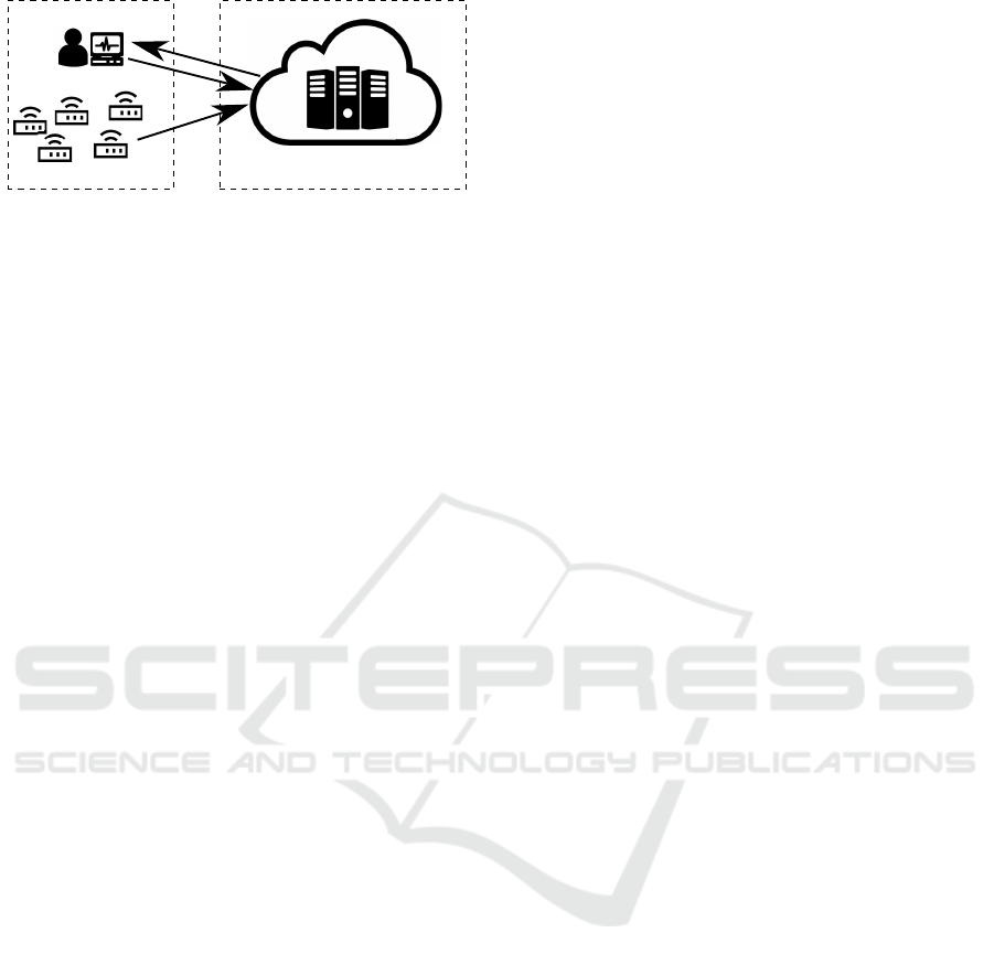
Figure 1: Devices send data to the remote service provider

(server S) for storage and processing. The beneﬁciary,

which resides on the client side, receives the processing re-

sults, either periodically or upon issuing a speciﬁc query.

We propose a new approach to do regression in

untrusted remote infrastructures that does not depend

on a non-collusion assumption and is several orders

of magnitude faster than existing solutions based on

FHE. The key insight is that not all data necessarily

needs to be encrypted in many practical scenarios, and

this fact can be exploited to build efﬁcient regression

algorithms based on partially homomorphic encryp-

tion.

In this paper, two different regression scenarios

are considered, each keeping a different part of the

data unencrypted. In the ﬁrst scenario, we use inde-

pendent variables in plaintext and encrypted depen-

dent variables to train an encrypted model, based on

the algorithm provided by the client, that can be used

to compute encrypted dependent variables. Thus, in

this scenario, the provider learns what independent

variables are used to build the model but the provider

cannot make sense of the computed model, nor can

the provider learn anything about the computed de-

pendent variables. This scenario has a wide range of

practical applications. For example, public wind and

weather data (plain text independent variables) can be

used to predict operational points of wind farms and

solar plants (encrypted dependent variables), or elec-

tricity consumption can be used to predict prices on

the electricity market (or the other way round). Other

examples are the use of social media data for sen-

timent analysis and current pricing information for

stock market prediction.

Of course, there are just as many applications

where both independent and dependent variables are

conﬁdential. In this case, we propose to keep the

model in plaintext, and use the encrypted conﬁdential

data (both independent and dependent variables are

encrypted) to train this model. The model can then be

used to compute encrypted dependent variables. The

provider cannot deduce anything about the computed

dependent variables since they are encrypted with the

client’s key to which the provider has no access.

The contributions of this work are the follow-

ing. We propose approaches to perform regression

analysis in a privacy-preserving manner where data

and model are partially encrypted and only one server

is needed (i.e., a non-collusion assumption is not

necessary). An additively homomorphic encryption

scheme is sufﬁcient to implement these approaches.

To illustrate our mechanisms, we use linear regression

and provide a comparative evaluation using both real-

world and synthetic data sets. The evaluation shows

that our mechanisms are fast enough for many prac-

tical use cases by computing a model in the order of

seconds and predictions in the order of milliseconds.

Furthermore, the evaluation reveals that our approach

is considerably faster than any state-of-the-art imple-

mentation based on two-server solutions or FHE: we

can achieve a speed-up of 4 orders of magnitude or

more. Thus, tremendous performance gains are feasi-

ble when sacriﬁcing full data privacy preservation by

encrypting only the most crucial parts of the data.

The paper is structured as follows. Our model is

explained in detail in §2. Our mechanisms are pre-

sented and evaluated in §3 and §4, respectively. Re-

lated work on privacy-preserving machine learning

and regression in particular is summarized in §5. Fi-

nally, §6 concludes the paper.

2 MODEL

In an industrial setting, there are three parties involved

in machine learning tasks: the devices generating the

data, the service provider carrying out demanding

computations and the beneﬁciaries receiving the re-

sults of the computations. Our model of this setting is

depicted in Figure 1. For simplicity, we consider the

parties providing the data and requiring the results as

one party, i.e., devices and beneﬁciary are merged in

a client role C. We assume that all clients subsumed

in client C belong to the same trust domain, i.e., they

are allowed to learn the same information in any pro-

cessing task. The service provider, on the other hand,

remains a separate untrusted party denoted by S. S is

assumed to be honest-but-curious, i.e., it follows the

protocol and does not attempt disruptions or fraud.

Moreover, we assume that S cannot break the used

cryptographic schemes for keys of reasonable length.

Typically, the devices are equipped with resource-

constrained hardware, both in terms of computational

power and storage, while the beneﬁciaries have more

computational resources, e.g., in the form of a pow-

erful computer, and the service provider has signiﬁ-

cantly more computational resources and storage ca-

pacity in the form of a computer cluster or a data cen-

ter. Therefore, the data produced at the client C must

SECRYPT 2017 - 14th International Conference on Security and Cryptography

256

be transferred to and stored at the service provider S.

In addition, as much computational load as possible

must be shifted from C to S. In particular, we con-

sider two tasks, which must be executed primarily by

S, a training task and a prediction task.

The training task consists of ﬁtting a model to data

according to a function f. The data consists of m

samples, where each sample i contains a vector x

(i)

n features—the independent variables—and a scalar

(i)

, which constitutes the dependent variable. Let

X and y denote the matrix and the vector of all in-

dependent and dependent variables, respectively. The

model computed in the training task is θ = f (X, y).

The prediction task uses the model θ, computed

from known X and y, to predict the dependent vari-

able for new independent variables. More formally,

a prediction is computed through some function g

based on the vector x of independent variables and

the model θ: y = g(x, θ). In this paper, we focus

on functions f and g that can be approximated by a

bounded-degree polynomial.

In order to ensure that the untrusted provider S

learns as little as possible during the course of the

computation, data is encrypted before being transmit-

ted to S. Note that there are fundamentally different

approaches such as obfuscating data, e.g., by adding

noise according to some predeﬁned distribution. We

assume that the unaltered data must be stored in the

database, which prohibits the use of such schemes.

This situation occurs quite naturally when the remote

infrastructure is also used as a data archive, which

may be a regulatory necessity. When using asymmet-

ric cryptography, only the beneﬁciary C needs access

to the secret key whereas the data generating devices

solely use the public key for encryption. Our algo-

rithms require that the encryption scheme be addi-

tively homomorphic, i.e., sums can be computed on

encrypted values directly without access to the (de-

cryption) key. Formally, let [v]

denote the cipher

text corresponding to the plaintext value v encrypted

with key k. An encryption scheme is called addi-

tively homomorphic if there is an operator ⊕ such

that [v

]

⊕ [v

]

is an encryption of v

+ v

for

any key k and values v

and v

Since it is always

clear from the context which key is used, we omit the

index and simply write [v]. In addition, we require

homomorphic multiplication of an encrypted number

with a plaintext factor, resulting in an encryption of

the product of the encrypted number and the factor.

Several additively homomorphic encryption schemes

support this operation. For ease of exposition, we use

Note that there may be many valid ciphertexts (en-

crypted values) corresponding to the same plaintext value

so we cannot assume that [v

]

⊕ [v

]

= [v

+ v

]

homomorphic operators implicitly whenever at least

one operand is encrypted, e.g., [v

] + [v

] and v

]

denote the homomorphic addition (where both terms

are encrypted) and multiplication (where one of the

terms is encrypted), respectively.

Our algorithms to train a model and predict depen-

dent variables are based on the exchange of plaintext

and ciphertext messages between S and C and local

computation at the two parties. The primary complex-

ity measure of an algorithm is the computational com-

plexity, which is the number of basic mathematical

operations, either on plaintext or on ciphertext, that

need to be carried out. As mentioned earlier, the goal

is to minimize the effort of C. Additionally, we dis-

cuss how many encrypted and plaintext values must

be exchanged during the execution of the algorithm.

3 PRIVACY-PRESERVING

LINEAR REGRESSION

3.1 Basic Concepts

Linear regression is a method to compute a model

θ representing a best-ﬁt linear relation between x

(i)

and y

(i)

, i.e., we get that x

(i)

· θ = y

(i)

+ e

(i)

for all i ∈ {1, . . . , m}, where e

(i)

are error terms.

More precisely, θ should minimize the cost function

J(θ) :=

i=1

(i)

· θ − y

(i)

)

. The model θ

can then be used to predict y for vectors x that are

obtained later by computing x · θ.

There are two commonly used approaches to com-

pute θ in such a way that the cost function J(θ)

is minimized. The ﬁrst approach solves the normal

equation θ = (X

−1

y, the second one uses

gradient descent. In the gradient descent-based ap-

proach, θ is updated iteratively, using the derivative

of J(θ), until J(θ) converges to a small value as fol-

lows:

:= θ

− α

∂J

∂θ

= θ

− α

i=1

(i)

· θ − y

(i)

(1)

The parameter α inﬂuences the rate of convergence.

The approach with normal equation requires the in-

version of an n × n-matrix. Therefore, gradient de-

scent can be signiﬁcantly faster when the number of

features is large.

For gradient descent to work well, features should

have a similar scale. For the sake of simplicity, we

assume that numerical values in the data are normal-

ized, i.e., the mean is shifted to 0 and all values are

scaled to be in the range [−1, 1]. We further assume

that the mean µ or at least an approximate bound

Privacy-preserving Regression on Partially Encrypted Data

257

is known. Given (the approximation of) µ, the de-

vices can easily perform this normalization by setting

←

−µ

max{x

max

−µ,µ−x

min

}

for all i ∈ {1, . . . m}.

This feature scaling and fractional numbers in

general pose a problem when working with encrypted

data as most encryption schemes operate on integers

in a ﬁnite ﬁeld. We address this problem by trans-

forming the values into ﬁxed-point numbers before

they are encrypted and processed. To this end, we

introduce an approximation step, where each value is

multiplied with a large factor and then rounded to the

closest integer, before encrypting the data. The mag-

nitude of the factor has an impact on the achievable

precision, as we will discuss in more detail in §4. For-

mally, we write

ˆx := approximate(x, λ),

where x is the independent variable, λ is the factor

that is multiplied with x, and ˆx is the rounded re-

sult. This subroutine approximate can naturally

be extended to take a vector or matrix as input by

applying the subroutine to each scalar in the vector

or matrix. We will use this extended deﬁnition of

the subroutine in our algorithms. The loss in preci-

sion becomes negligible when λ is large enough. For-

mally, if c = f(a, b) for some function f, we write

ˆc ' f(ˆa,

b). In other words, we almost get the same

result when applying the subroutine to the result of

a computation as when carrying out the computation

with approximated inputs. We further write ˆc ' λc,

which states that ˆc is λ times larger up to rounding.

As mentioned before, we consider encryption

schemes that support homomorphic multiplication of

encrypted values with plaintext values. Again, such a

multiplication is only possible with plaintext integers

but our mechanisms require the capability to multi-

ply encrypted values with arbitrary rational numbers.

There are two options to provide this operation. The

ﬁrst option entails a loss of precision by converting

the factor into a ﬁxed-point number using again the

approximation subroutine. The second option is to in-

volve the client in the computation by asking it to de-

crypt the value, carry out the multiplication, round the

result to the nearest integer, and send the encrypted re-

sult back to S. We use both options in our algorithms,

carefully selecting between them to minimize the pre-

cision loss and the communication and computational

load on the client.

3.2 Algorithms

All our proposed algorithms allow the client C to pre-

process each sample separately. In other words, the

algorithms can be used in environments with multiple

Client Server

X, [ŷ], λ

]

] := M[

] − T[ŷ]

:= α/m·r

]

[

] := [

] − [d

]

] := M[

] − T[ŷ]

]

:= α/m·r

]

...

M := approximate(X

X,λ)

T := approximate(X

,λ)

Figure 2: Encrypted θ&y using gradient descent.

data sources, without requiring them to communicate

with each other. Some of our algorithms involve C in

the computation as outlined in the previous section.

As discussed in §1, we consider two different sce-

narios, each scenario encrypting a different set of pa-

rameters.

1) Encrypted θ&y: The matrix of independent vari-

ables X is provided in plain text whereas the

model θ and the vector of dependent variables y

are encrypted.

2) Encrypted X&y: Both the matrix of independent

variables X and the vector of dependent variables

y are encrypted but the model θ is in plaintext.

For Scenario 1), we propose three methods to

compute θ in encrypted form: The ﬁrst one uses gra-

dient descent and is thus particularly useful for sce-

narios where X contains many features. The sec-

ond method solves the normal equation, and the third

method requires the client to do some preprocessing

of the data in order to speed up the computation on the

server. After discussing these methods, we present an

algorithm for Scenario 2) based on gradient descent.

3.2.1 Encrypted θ&y using Gradient Descent

Initially, C sends the independent variable matrix X

in plaintext and the corresponding dependent variable

vector y in encrypted approximate form (



ˆy



) to S.

Thus, C sends mn plaintext values and m encrypted

values. S then applies Equation (1) iteratively on the

data. To this end, S performs the approximation for

X and X

M := approximate(X

X, λ)

T := approximate(X

, λ)

Subsequently, S computes





:= M





− T



ˆy



where the initial model θ

is set to a suitable starting

vector in encrypted form. In the next step, S sends

] to the client, which decrypts it, applies the multi-

plication with α/m and sends back the result. This

operation is assigned to the client since α/m is a num-

SECRYPT 2017 - 14th International Conference on Security and Cryptography

258

Algorithm 1: TRAINING: Encrypted θ&y using nor-

mal equation.

Input: X,



ˆy



, λ

Output:





1 A := approximate((X

−1

, λ)





:= A



ˆy



3 return





ber close to zero if there are many samples, and thus

the precision loss by carrying out this multiplication

on S can be signiﬁcant. These two steps are repeated

K times (or until the client decides that the value is

small enough). This scheme is illustrated in Figure 2.

It is easy to see that the model is updated accord-

ing to Equation (1). In each iteration, 2n ciphertext

values are transmitted from S to C and back. Thus,

O(Kn) ciphertexts are exchanged during gradient de-

scent. Overall, S must perform O(Kmn) homomor-

phic operations and O(Kn) operations on plaintext,

whereas C carries out O(Kn) plaintext, encryption,

and decryption operations.

3.2.2 Encrypted θ&y using Normal Equation

The second approach solves the normal equation on

S directly. In this case, no interaction with the client

is necessary after receiving X and



ˆy



Given X and λ, S ﬁrst computes (X

−1

and applies the subroutine approximate. S can

then use this matrix together with



ˆy



to compute





see Algorithm 1. This computation is obviously cor-

rect in principle but there is a loss in precision due to

the approximation.

Overall, O(mn

+ n

2.373

) plaintext operations

are performed to compute A. The second term

is the complexity of inverting X

X for optimized

variants of the Coppersmith-Winograd algorithm.For

problems with a large number of features, the inver-

sion can be computed by other methods, e.g., with LU

decompositions. In addition, O(nm) homomorphic

operations (additions of ciphertexts and multiplica-

tions of ciphertexts with plaintext values) are needed

to compute





. If n is relatively small, e.g., 1000 or

less, the homomorphic operations are likely to dom-

inate the computational complexity as they are typi-

cally several orders of magnitude slower than equiv-

alent operations in the plaintext domain. A detailed

analysis is given in §4.

3.2.3 Encrypted θ&y with Preprocessing

The third approach is also based on solving the nor-

mal equation but reduces the number of homomorphic

operations on S for the case when the number of sam-

ples m is greater than the number of features n. This

reduction is achieved by preprocessing the data on the

client side as follows. As before, C sends the matrix

X to S. However, instead of sending



ˆy



, C computes

:= X

(i)

, where X

(i)

denotes the i

row of

X, and transmits





for each i ∈ {1, . . . , m}.

The server S then computes

A := approximate((X

−1

, λ).

Next, it sums up the vectors





for all i ∈

{1, . . . , m} homomorphically, which yields the en-

crypted vector





, where b = X

y. Finally, θ is

computed by multiplying A and





homomorphi-

cally. The algorithm is summarized in Algorithm 2.

The homomorphism with respect to addition im-

plies that

b =

i=1

(i)

ˆy

(i)

= X

ˆy.

Thus, Algorithm 2 solves the (approximate) normal

equation for θ correctly by multiplying A and





. If

m > n, the advantage of Algorithm 2 as opposed to

Algorithm 1 is that the number of homomorphic mul-

tiplications on S is reduced from O(nm) to O(n

Conversely, C must perform O(mn) additional oper-

ations to compute the vectors





, . . . ,





. In ad-

dition to transmitting the plaintext matrix X, C also

sends these m n-dimensional vectors, i.e., O(mn)

values are sent in total.

Since each vector [

bi] is sent individually, using

the algorithm in a setting with multiple clients is

straightforward. If there is only one client that holds

X and y locally, the algorithm can be optimized:

The client computes b = X

y directly and sends





to S. In this case, the client must only encrypt

b, i.e.,

n values in total, in contrast to encrypting all vectors

, which requires the encryption of nm values.

Moreover, S would not have to compute





3.2.4 Encrypted X&y using Gradient Descent

We now consider the scenario where X and y are

encrypted and the model θ is computed in plain-

text. Solving the normal equation directly involves

the multiplication of elements of X and y, which

is not possible using an additively homomorphic en-

cryption scheme. Gradient descent cannot be used

directly either because X

must be multiplied with

terms containing X and y. However, it is possible to

use gradient descent when the client performs some

preprocessing on the data: For each sample i, the

Privacy-preserving Regression on Partially Encrypted Data

259

Algorithm 2: TRAINING: Encrypted θ&y with pre-

processing.

Input: X, λ, {





, . . . ,





}

= X

(i)

)

Output:





1 A := approximate((X

−1

, λ)





i=1









:= A





4 return





client prepares a vector [

], where b

= X

(i)

and matrix [

], where A

= X

(i)

, and trans-

mits them to S.

As in §3.2.1, the initial model θ

is set to a suit-

able starting vector. In order to support values smaller

than 1 in the model, θ

is scaled by λ. S sums up

all received encrypted vectors [

] and multiplies the

sum with λ homomorphically, resulting in the en-

crypted vector [

b]. The encrypted matrices [

] are

also summed up homomorphically, which yields the

encrypted matrix [

A]. Vector [

b] and matrix [

A] are

used in each iteration i as follows: S sends









i−1

−





to C, where it is decrypted and mul-

tiplied with α/m before being converted again to an

integer using the subroutine approximate. The re-

sult

is sent back to S. The updated model θ

computed by subtracting

from θ

i−1

. The algorithm

is depicted in Figure 3.

Again, due to the homomorphic property of the

encryption scheme, we have that

A =

i=1

' λ

i=1

= λX

X (2)

b = λ

i=1

' λ

i=1

= λ

y, (3)

and thus

(

Aθ

i−1

−

(2),(3)

' X

Xθ

i−1

− X

where r

denotes the correct difference between the

two terms on the right-hand side. Hence, the algo-

rithm implements gradient descent correctly.

As far as the computational complexity is con-

cerned, S carries out O(mn

+ Kn

) homomorphic

additions and O(Kn

) homomorphic multiplications.

At the beginning, the client sends m(n

+ n) en-

crypted values. n encrypted values are exchanged in

each iteration. C has to decrypt them, carry out a mul-

tiplication and convert them to integers before send-

ing them back to S. Thus, O(mn

+ Kn) values are

Client Server

[Â

],..., [Â

], [b

],..., [b

],λ

]

] := [Â]

− [b

]

:= α/m·r



:= 

− d

] := [Â]

− [b

]

:= α/m·r

...

[Â] := Σ

[Â

]

] := λΣ

]

Figure 3: Encrypted X&y using gradient descent.

exchanged in total. Note that S learns not only the

ﬁnal model but also all intermediate models. It de-

pends on the use case whether this information leak-

age is acceptable. In other words, depending on the

data, S may or may not be able to extract information

from these models. In either case, it cannot directly

use them as they produce encrypted predictions.

3.2.5 Prediction

Having computed the model, the second fundamental

task is to predict y given a new input vector x. In Sce-

nario 1), x is not encrypted, so S can get the encrypted

prediction by computing [y] = x[θ]. Likewise, in Sce-

nario 2), the model θ is not encrypted, therefore S can

compute [y] = [x]θ. In both scenarios, S needs O(n)

homomorphic operations to compute a prediction.

3.3 Scalability

After having introduced the basic methods of our ap-

proach, we now describe optimizations, for both the

client and the server.

3.3.1 Packing

While most computational work is ofﬂoaded to the

server, the client is required to carry out many encryp-

tion and decryption operations in all proposed algo-

rithms. Since decryption is the most expensive oper-

ation, we will now discuss how we reduce the num-

ber of decryption operations at the client using a tech-

nique called packing (Brakerski et al., 2013; Ge and

Zdonik, 2007; Nikolaenko et al., 2013). The server

S packs multiple ciphertexts that must be sent to the

client into a single ciphertext by repeatedly shifting

and adding them, which can be done without knowl-

edge of the decryption key. However, S must know

how many bits are used to encode a single plain-

text. The client can then recover the plaintexts by

SECRYPT 2017 - 14th International Conference on Security and Cryptography

260

decrypting the ciphertext and extracting each individ-

ual plaintext by shifting and applying a bit mask. For

example, for a key size of 2048 bit and 32-bit plain-

texts, up to 64 ciphertexts can be packed, reducing

the number of decryptions by the same factor. This

feature is used in both gradient-descent based algo-

rithms, where S sends the encrypted vector [r

] in

each iteration.

3.3.2 Iterative Model Computation

In many application scenarios, the client sends a

stream of samples to the server, which in turn is sup-

posed to update the computed model accordingly ().

Our approaches can be adapted easily to accommo-

date such requirements. E.g., the gradient-descent

based algorithm for Encrypted θ&y can be modiﬁed

as follows: instead of sending X and



ˆy



, the client

sends x

(i)

and



ˆy

(i)



separately for each i. The server

then updates M and T based on the new values (a fast

operation since X is not encrypted), computes





and sends it back to the client. The client computes





and returns it to the server, possibly together with

the next sample. Similarly, in Algorithm 1 and Algo-

rithm 2 the matrix A and vector





can be updated ef-

ﬁciently after receiving each sample. This also holds

for Encrypted X&y, where









and





can be

computed efﬁciently for each new sample.

Depending on the application, it might also make

sense for the client to send samples in batches; the

iterative approach outlined above can be adapted for

batched samples as well. The computation complex-

ity on the server can be reduced using optimization

methods decreasing the frequency with which a new

model is computed (Strehl and Littman, 2008) or a

recursive approach that assigns more weight to recent

samples (Gruber, 1997). In our evaluation, we inves-

tigate the performance of our methods without such

optimizations to gain an understanding of their basic

behavior in different scenarios.

4 EVALUATION

4.1 Experimental Setup

We use several data sets with different numbers of

samples and features to evaluate the performance.

Real-world data sets: In order to enable other re-

searchers to compare their methods to ours, we have

chosen 8 publicly available data sets.

In this paper,

we focus primarily on two representative data sets:

See https://archive.ics.uci.edu/ml/datasets/.

Set 1 contains data from a Combined Cycle Power

Plant (CCPP) with 9568 samples and 4 features. Set

2 is called Condition Based Monitoring (CBM) with

11,934 samples and 17 features. A summary of our

results for the other 6 data sets is provided as well.

Furthermore, we also generate synthetic data to ana-

lyze the impact of the number of samples and features

on the computational complexity.

Synthetic data sets: We generated synthetic data

sets with 10 to 80 features and 1000 to 64’000 sam-

ples, where the elements of X are ﬂoating point val-

ues chosen uniformly at random between 0 and 1 and

y is computed for a model vector θ with randomly

chosen ﬂoating point numbers and some noise.

We use the additively homomorphic Paillier en-

cryption scheme (Paillier, 1999) in our implementa-

tion, which supports the required homomorphic oper-

ations. In this encryption scheme, a homomorphic ad-

dition corresponds to a multiplication (of ciphertexts),

while a homomorphic multiplication corresponds to

an exponentiation, where the plaintext factor is the

exponent. All homomorphic operations are carried

out modulo a large number. The most expensive op-

erations, encryption and decryption, have been op-

timized using standard tricks such as precomputing

random factors and working in a subgroup generated

by an element of order αn (Jost et al., 2015).

We implemented our algorithms in C++ using the

library NTL

and used 2048-bit encryption keys, cor-

responding to a 112-bit security level (Catalano et al.,

2001).

For comparison, we implemented the gradient de-

scent and matrix inversion methods for unencrypted

data using the Armadillo library

. We ran the tests

on a computer with an Intel Core i5-2400 CPU at 3.1

GHz and 24GB of RAM, running Ubuntu 14.04.

4.2 Precision

We normalized the data in the data sets as described

in §3.1. The number of bits used to represent real val-

ues as ﬁxed-point integers is a compromise between

precision and overhead in storage and computation

time. In order to better understand this trade-off, we

measured the precision error, deﬁned as the Euclidean

norm of the difference between θ obtained with ap-

proximated values and θ obtained with arbitrary pre-

cision ﬂoating point values, using different numbers

of bits for the approximation. The precision error

when computing with 64-bit ﬂoating point numbers is

in the order of 10

−71

for CBM and 10

−72

for CCPP.

We found that this level of precision can be matched

See http://www.shoup.net/ntl/.

See http://arma.sourceforge.net/.

Privacy-preserving Regression on Partially Encrypted Data

261

Table 1: Running times for computing the model without encryption. The ﬁrst number is for the CCPP data set and the second

one in parentheses for the CBM data set.

Training plaintext, gradient descent, K=10 plaintext, normal equation

Server training total [ms] 11 (24) 0.15 (1.4)

Table 2: Running times and overhead factors for computing the model with Paillier encryption. The ﬁrst number is for the

CCPP data set and the second one in parentheses for the CBM data set.

Training Encrypted θ&y Encrypted θ&y Encrypted θ&y Encrypted X&y

gradient descent normal equation preprocessing gradient descent

K=10 K=10

Client prep./sample [ms] 1.16 (1.98) 1.14 (1.99) 5.02 (17.731) 26.23 (106.23)

Client training/iter. [ms] 9.05 (20.11) - - 118.23 (143.91)

Server training/iter. [ms] 187.55 (949.24) - - 411.30 (3713.22)

Server training total [ms] 1966.01 (9693.32) 1553.66 (8748.05) 116.42 (571.23) 5550.35 (38314.80)

Server overhead 179 (404) 10,371 (6,249) 799 (408) 3,483 (1583)

using 50 bits for the approximation. Since measure-

ments themselves contain errors, such a high preci-

sion is typically not necessary. Therefore, we decided

to use 30 bits, which corresponds to precision errors

in the order of less than 10

−35

. Note that 20 bits are

used in relevant related work (Graepel et al., 2012;

Nikolaenko et al., 2013).

4.3 Time

We present results for the time needed to compute

the model and make predictions as averages over 100

runs. First, we analyze the performance of our algo-

rithms on real-world data sets. Afterwards, we study

how the two main parameters—the number of sam-

ples and features in the data set—affect performance

using randomly generated data.

4.3.1 Analysis Using Real-World Data Sets

The times for computing the model (training task)

without encryption and with encryption are given in

Table 1 and Table 2, respectively. Each method from

§3.2 is presented in a separate column, gradient de-

scent was performed for K=10 iterations. The rows

indicate the following: “Client preparation per sam-

ple” shows the time the client needs to preprocess and

encrypt a single sample, whereas “Client training per

iteration” shows how much time is spent at the client

to compute the update to the model in each gradi-

ent descent iteration. “Server training per iteration”

shows the time spent at the server for a single gradient

descent iteration, and “Server training total” shows

the total time needed by the server. This total time

includes the time spent at the client when performing

0.5

1.5

10 20 30 40 50 60

Time for 1 prediction (in ms)

Number of bits for fixed point representation

CCPP with [X]

CCPP with [θ]

CBM with [X]

CBM with [θ]

Figure 4: Running time to compute one prediction for dif-

ferent numbers of bits used to approximate real numbers.

operations on behalf of the server in each gradient de-

scent iteration. However, the “Client per sample” time

is excluded as it is dominated by the time to encrypt

samples, which we do not consider a part of comput-

ing the model. “Server overhead” shows the overhead

factor, which is the ratio between the “Server training

total” times in Table 2 and Table 1.

The time for predictions is shown in Table 3. For

the scenario when X and y are encrypted, it com-

prises the time for encryption at the client and the time

for computing the prediction on the server. Recall that

we always use 30 bits to encode input values as ﬁxed-

point numbers. It is important to understand how the

encoding affects performance. Figure 4 depicts the

dependence of the time required to make a prediction

on the number of bits used for the approximation.

As mentioned before, we also ran our algorithms

on six other data sets. Since these experiments did not

yield substantially different results, we omit a detailed

analysis and present a short summary in Table 4 and

SECRYPT 2017 - 14th International Conference on Security and Cryptography

262

Table 3: Running times and overhead factors for predictions. The ﬁrst two column use Paillier encryption, the last column no

encryption. The ﬁrst number is for the CCPP data set and the second one in parentheses for the CBM data set.

Prediction Encrypted θ&y Encrypted X&y plain text

Client [ms] 0.523 (0.525) 4.631 (4.678) -

Server [ms] 0.244 (0.934) 0.347 (0.376) 0.000224 (0.0000711)

Server overhead [×10

] 3.440 (4.176) 5.291 (1.552) -

Table 4: Average server overhead of training for 6 additional data sets (separate numbers for each proposed algorithm).

Data set Training

Name Features Samples Encr. θ&y Encr. θ&y Encr. θ&y Encr. X&y

grad. descent normal eq. preprocessing grad. descent

Auto-mpg 8 394 558 16,307 2,957 13,415

Forestﬁre 10 518 533 14,414 2,054 15,156

BCW 10 684 711 11,921 1,036 15,280

Concrete 14 1031 323 4,142 467 4,460

Red Wine 12 1600 678 9,767 935 9,533

White Wine 12 4899 386 5,118 361 2,549

Table 5. The table contains the number of features

and samples for each data set. Moreover, it shows the

server overhead for each of the four proposed algo-

rithms when training the model and the server over-

head to compute predictions for both considered sce-

narios (encrypting θ and y or X and y).

4.3.2 Analysis Using Synthetic Data Sets

Since all cryptographic operations (encryption, de-

cryption, and homomorphic operations) take roughly

the same amount of time independent of the actual

data values, the performance depends primarily on a)

the chosen algorithm and b) the number of features

and samples in the data set.

It is thus worth investi-

gating how varying the number of features and sam-

ples affects the performance of each algorithm. To

this end, we generated random data sets with F fea-

tures and S samples where F ∈ {10, 20, 40, 80} and

S ∈ {1000, 2000, 4000, . . . , 32000}. As before, we

are interested in the overhead for training and pre-

dicting. Ideally, the running times increase in a simi-

lar fashion when increasing the number of features or

samples for both unencrypted and encrypted data. In

other words, the server overhead remains constant re-

gardless of the dimensions of the input. Figure 5 and

Figure 6 show the running time for the training phase

and predictions when increasing the number of sam-

ples and features, respectively. The number of fea-

tures is set to 10 in Figure 5, and 1000 samples are

Note that the time for encryption per value is also more

or less constant as we always use 30 bits to encode data

values.

used in Figure 6.

4.4 Discussion

In comparison to training a model without encryption,

the overhead factor is between 179 and 600 for gradi-

ent descent when y and θ are encrypted and between

2500 and 15000 when X and y are encrypted. Note

that the overhead decreases with higher numbers of

samples. When solving the normal equation, the over-

head is roughly between 5000 and 17000 without pre-

processing and drops to about 300 to 3000 with pre-

processing. Thus, solving the normal equation is sub-

stantially faster for a small number of features than

gradient descent. What is more, the overhead on the

server can be lowered by an order of magnitude by

imposing some work on the client for preprocessing

or divisions.

The overhead for predictions is higher. However,

these operations are typically performed on single

samples rather than bulk data and therefore the ab-

solute time per prediction is still fairly small and ac-

ceptable for practical use. More importantly, the com-

munication cost is often several orders of magnitude

larger than the cost of prediction, which implies that

the end-to-end slow-down is negligible.

When y and θ are encrypted our algorithms com-

plete training the model in less than 10 seconds on

all datasets. For the use case where X and y are en-

crypted, the largest dataset requires 38 seconds for

training. Predictions can be executed in the subsec-

ond range. We conclude that the running times of our

methods on both data sets are within a range accept-

Privacy-preserving Regression on Partially Encrypted Data

263

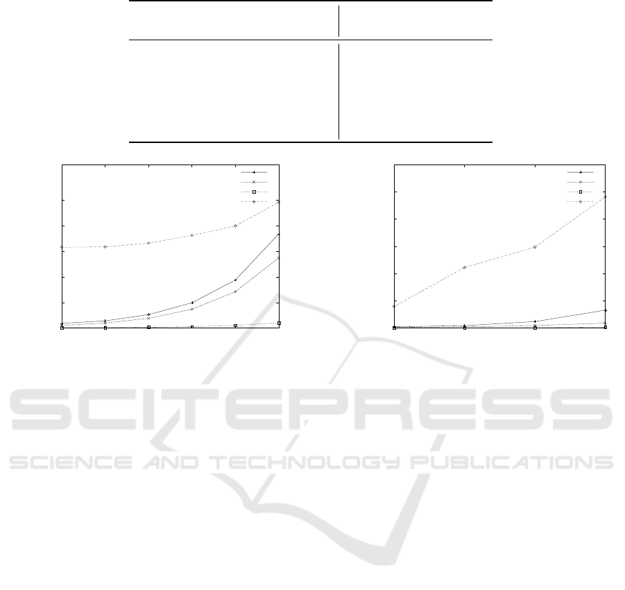
Table 5: Average server overhead of prediction for 6 additional data sets (Encrypted θ&y and Encrypted X&y).

Data set Prediction

Name Features Samples Encr. θ&y Encr. X&y

Auto-mpg 8 394 2,640 4,840

Forestﬁre 10 518 3,657 6,479

BCW 10 684 3,818 6,835

Concrete 14 1031 1,640 2,975

Red Wine 12 1600 3,465 6,120

White Wine 12 4899 3,427 6,327

5000

10000

15000

20000

25000

1000 2000 4000 8000 16000 32000

Running time [ms]

Number of samples

Encr. θ&y grad. descent

Encr. θ&y norm. equation

Encr. θ&y preprocessing

Encr. X&y grad. descent

Figure 5: The running time for each algorithm to train

the model in both considered scenarios is given for

1000, 2000, 4000, . . . , 32, 000 samples. Each data set con-

tains 10 features.

able for practical use.

Encrypted θ&y methods applying the normal

equation directly with or without preprocessing ex-

hibit the following beneﬁts: (i) No interaction with

the client is needed during the computation of the

model. (ii) The results are very accurate and the user

does not need to decide on parameters such as learn-

ing rate and number of iterations. This makes the

process of choosing parameters easier—in the case of

gradient descent, a wrong learning rate could result in

the method not converging. On the contrary, the com-

plexity and feasibility of all methods incorporating

gradient descent strongly depends on the choice of pa-

rameters, particularly the learning rate α and the num-

ber of iterations K. If α is too large, the method does

not converge. If it is too small, many iterations are re-

quired to achieve an acceptably small error J(θ). The

number of iterations could be decreased by automati-

cally tuning α between iterations based on the rate at

which the error J(θ) is decreasing. This optimization

would require sending additional encrypted values to

the client in order to compute the error of the updated

model. It depends on the data whether this overhead

is less than the time saved by reducing the number of

iterations. The gradient descent approaches perform

particularly well on larger data sets, where the num-

20000

40000

60000

80000

100000

10 20 40 80

Running time [ms]

Number of features

Encr. θ&y grad. descent

Encr. θ&y norm. equation

Encr. θ&y preprocessing

Encr. X&y grad. descent

Figure 6: The running time for each algorithm to train the

model and for computing predictions in both considered

scenarios is given for 10, 20, 40, 80 features. Each data set

contains 1000 samples.

ber of samples is in the order of ten thousand features.

When looking at the synthetic data sets (see Fig-

ure 5 and Figure 6) we can observe the behavior of

our methods for a growing number of samples. In the

plotted range all running times increase roughly lin-

early both with the number of samples and with the

number of features (note that the x-axis of the plots

is in log-scale). The number of features has a large

impact on the running times, thus it is best to keep

the number of features small, which can typically be

achieved using techniques such as principal compo-

nent analysis. We can further clearly see the differ-

ence between all the proposed algorithms with respect

to running time. In particular, the scenario when X is

in plaintext yields signiﬁcantly smaller running times.

Recall that optimizations are possible with iterative

processing as described in §3.3.2.

Using a leveled or fully homomorphic encryption

scheme would allow us to encrypt X, y, and θ. How-

ever, communication with the client would still be

necessary for the gradient descent iteration steps be-

cause the known leveled and fully homomorphic en-

cryption schemes do not support division. This lim-

itation further entails that an approach based on the

normal equation is hard to implement. If X, y, and

θ must be encrypted, the multiplication of two ci-

SECRYPT 2017 - 14th International Conference on Security and Cryptography

264

phertext values is necessary for linear regression. Li-

braries such as HElib

offer this operation, yet the

size of messages and keys and also the running time

are large. For example, one could apply the method

of Encrypted X&y with θ encrypted. In this case,

the most costly operation per gradient descent itera-

tion step is the multiplication of an encrypted n-by-n

matrix with an encrypted vector of length n. Imple-

menting this as proposed in (Halevi and Shoup, 2014),

gives a lower bound of the running time per iteration

of 25s for CBM and 8s for CCPP with HElib’s default

conﬁguration for 32-bit plaintext integers. Thus, this

method is at least 10,400 (178,000) times slower than

plaintext operations for CCPP (CBM).

With a naive encoding of numbers (e.g., HElib’s

current encoding), around 9GB of encrypted data

would need to be sent for the training task with CCPP.

Different methods to compute the inverse of a matrix

would need to be considered to decrease the commu-

nication cost. These results clearly show the substan-

tial difference in performance when either X or θ is

left in plaintext as opposed to encrypting X, y, and θ.

5 RELATED WORK

Privacy-preserving techniques for outsourcing ma-

chine learning tasks received a lot of attention in

a variety of scenarios. In this section, we discuss

the most closely related approaches for regression.

To the best of our knowledge, existing work em-

ploys either protocols with additional parties, e.g.,

two-server or multi-party-computation solutions un-

der non-collusion assumptions, e.g., (Damgard et al.,

2015; Du et al., 2004; Hall et al., 2011; Karr et al.,

2009; Nikolaenko et al., 2013; Peter et al., 2013;

Samet, 2015), or protocols based on fully homomor-

phic encryption, e.g., (Graepel et al., 2012; Bost et al.,

2014).

Nikolaenko et al. consider the scenario where both

the dependent and independent variables are conﬁ-

dential and the model is computed in plaintext (Niko-

laenko et al., 2013). They propose a two-server solu-

tion for ridge regression using the partially homomor-

phic Paillier cryptosystem (Paillier, 1999) and garbled

circuits (Goldwasser et al., 1987; Yao, 1986). Under

the assumption that the two servers do not collude,

they provide methods for the parameter-free Cholesky

decomposition to compute the pseudo inverse. On

the same data sets and on data sets of similar di-

mensions, their approach can take 100-1000 times

longer, despite the fact that they use shorter keys.

See https://github.com/shaih/HElib.

Other solutions for the privacy-preserving computa-

tion with multiple servers include encryption schemes

with trapdoors (Peter et al., 2013), multi-party-

computation schemes or shared data, e.g., (Damgard

et al., 2015; Du et al., 2004; Hall et al., 2011; Karr

et al., 2009; Samet, 2015).

Graepel et al. present an approach enabling the

computation of machine learning functions as long as

they can be expressed as or approximated by a poly-

nomial of bounded degree with leveled homomorphic

encryption (Graepel et al., 2012), using the library

HElib based on the Brakerski-Gentry-Vaikuntanathan

scheme (Brakerski et al., 2012). They focus on binary

classiﬁcation (linear means classiﬁcation and Fisher’s

linear discriminant classiﬁer). Moreover, they assume

that it is known for two encrypted training examples

whether they are labeled with the same classiﬁcation

(without revealing which one it is). In contrast, we

apply simpler encryption methods that are several or-

ders of magnitude faster on the data set BCW. Bost

et al. consider privacy preserving classiﬁcation (pre-

dictions but no training) (Bost et al., 2014). They

combine different encryption schemes into building

blocks for the computation of comparisons, argmax,

and the dot product. These building blocks require

messages to be exchanged between the client and the

server, which is not necessary in the computation of

predictions with our algorithms.

6 CONCLUSION

We have proposed methods to train a regression

model and use it for predictions in scenarios where

part of the data and the model are conﬁdential and

must be encrypted. By exploiting the fact that not

everything is encrypted, our methods work with par-

tially homomorphic encryption and thereby achieve

a signiﬁcantly lower slow-down factor than state-of-

the-art methods applicable to scenarios where every-

thing must be encrypted. We have further presented

an evaluation of our methods on two data sets and

found the times needed to train a model and make

predictions small enough for practical use. Our main

contribution is hence addressing the problem in ways

that enable the use of partially homomorphic encryp-

tion and a single server. To the best of our knowledge,

there is no existing work for scenarios where indepen-

dent variables can be public and the dependent vari-

ables and model must be encrypted. The trade-offs of

the different methods we propose are of interest since

they are suitable for different dataset properties.

In this paper, we have provided the details for lin-

ear regression only; however, it is important to note

Privacy-preserving Regression on Partially Encrypted Data

265

that our techniques can be extended to functions that

can be approximated well by bounded-degree polyno-

mials. To this end, models are trained with powers of

the independent and dependent variables, where the

polynomials can be evaluated homomorphically by

multiplying the plaintext coefﬁcients of the bounded-

degree polynomials with powers of the sampled val-

ues and summing up the encrypted terms. While this

approach incurs additional cost in terms of computa-

tion and communication, it allows our techniques to

be applied to other problems, e.g., logistic regression

or support vector machines. Implementing privacy-

preserving equivalents of other algorithms based on

our techniques and evaluating their applicability in

practice is a valuable direction for future work.

REFERENCES

Bost, R., Popa, R. A., Tu, S., and Goldwasser, S.

(2014). Machine Learning Classiﬁcation over En-

crypted Data. Cryptology ePrint Archive, Report

2014/331.

Brakerski, Z., Gentry, C., and Halevi, S. (2013). Packed

Ciphertexts in LWE-based Homomorphic Encryption.

Brakerski, Z., Gentry, C., and Vaikuntanathan, V. (2012).

(Leveled) Fully Homomorphic Encryption Without

Bootstrapping. In Proc. 3rd Innovations in Theoret-

ical Computer Science (ITCS).

Catalano, D., Gennaro, R., and Howgrave-Graham, N.

(2001). The Bit Security of Paillier’s Encryp-

tion Scheme and its Applications. In Advances in

Cryptology—EUROCRYPT.

Damgard, I., Damgard, K., Nielsen, K., Nordholt, P. S., and

Toft, T. (2015). Conﬁdential Benchmarking based on

Multiparty Computation. Cryptology ePrint Archive,

Report 2015/1006.

Du, W., Han, Y. S., and Chen, S. (2004). Privacy-Preserving

Multivariate Statistical Analysis: Linear Regression

and Classiﬁcation. In Proc. SIAM International Con-

ference on Data Mining.

Ge, T. and Zdonik, S. (2007). Answering Aggregation

Queries in a Secure System Model. In Proc. 33rd

Conf. on Very Large Data Bases (VLDB).

Gentry, C. (2009). Fully Homomorphic Encryption Using

Ideal Lattices. In Proc. 41st Symposium on Theory of

Computing (STOC).

Goldwasser, S., Micali, S., and Wigderson, A. (1987). How

to Play any Mental Game, or a Completeness Theorem

for Protocols with an Honest Majority. In Proc. 19th

Symposium on the Theory of Computing (STOC).

Graepel, T., Lauter, K., and Naehrig, M. (2012). ML Con-

ﬁdential: Machine Learning on Encrypted Data. In

Information Security and Cryptology–ICISC.

Gruber, M. H. (1997). Statistical Digital Signal Processing

and Modeling.

Halevi, S. and Shoup, V. (2014). Algorithms in HElib. In

International Cryptology Conference.

Hall, R., Fienberg, S. E., and Nardi, Y. (2011). Secure Mul-

tiple Linear Regression Based on Homomorphic En-

cryption. Journal of Ofﬁcial Statistics, 27(4).

Jost, C., Lam, H., Maximov, A., and Smeets, B. J. M.

(2015). Encryption Performance Improvements of

the Paillier Cryptosystem. IACR Cryptology ePrint

Archive, 2015.

Karr, A. F., Lin, X., Sanil, A. P., and Reiter, J. P. (2009).

Privacy-Preserving Analysis of Vertically Partitioned

Data using Secure Matrix Products. Journal of Ofﬁcial

Statistics, 25(1).

Nikolaenko, V., Weinsberg, U., Ioannidis, S., Joye,

M., Boneh, D., and Taft, N. (2013). Privacy-

Preserving Ridge Regression on Hundreds of Millions

of Records. In Proc. IEEE Symposium on Security and

Privacy (S&P).

Paillier, P. (1999). Public-Key Cryptosystems Based on

Composite Degree Residuosity Classes. In Advances

in Cryptology—EUROCRYPT.

Peter, A., Tews, E., and Katzenbeisser, S. (2013). Efﬁ-

ciently Outsourcing Multiparty Computation Under

Multiple Keys. IEEE Transactions on Information

Forensics and Security, 8(12).

Samet, S. (2015). Privacy-Preserving Logistic Regression.

Journal of Advances in Information Technology, 6(3).

Strehl, A. L. and Littman, M. L. (2008). Online Linear

Regression and its Application to Model-based Rein-

forcement Learning. In Advances in Neural Informa-

tion Processing Systems.

Yao, A. (1986). How to Generate and Exchange Secrets.

In Proc. 27th Annual Symposium on Foundations of

Computer Science (FOCS).

SECRYPT 2017 - 14th International Conference on Security and Cryptography

266