Implementation and Evaluation of an On-demand Bus System

Sevket G

okay

1,2

, Andreas Heuvels

, Robin Rogner

and Karl-Heinz Krempels

1,2

Informatik 5 (Information Systems), RWTH Aachen University, Aachen, Germany

CSCW Mobility, Fraunhofer FIT, Aachen, Germany

Keywords:

Demand-responsive Transport, Dynamic Pickup and Delivery Problem, Vehicle Routing Problem with Time

Windows.

Abstract:

This work aims to develop and evaluate a dynamic bus system which abandons the concepts of a traditional

bus service like bus line, bus station and timetable. The resulting system supports bringing customers from

any location to any location, has a ﬂeet of buses the routes of which are updated repeatedly as requests arrive

and are accepted, and employs time windows in order to guarantee the desired pick-up and drop-off times of

customers. We propose a technical realization and evaluate its effectiveness by running simulations in which

traditional and dynamic systems are compared. Even though the operational cost and ﬁnancial efﬁciency

from a bus service provider’s perspective is not the focus of this evaluation, the preliminary results show that

both the provider and the customers might beneﬁt from an on-demand dynamic system. We also hint at the

feasibility of such a system in not only low-demand rural areas, but also high-demand urban regions.

1 INTRODUCTION

With the ever-improving technology landscape, tradi-

tional and existing systems are challenged with new

ideas that aim for optimization by making them more

intelligent. Transportation systems have always been

such a target and more speciﬁcally, public transporta-

tion beneﬁted immensely from advancements in IT

and mobile Internet becoming more widespread. The

operation of public transport bus services currently

bases on buses traveling along ﬁxed routes visiting

predeﬁned bus stops according to a ﬁxed timetable.

This is the product of efforts in public transportation

planning where many factors of all stakeholders are

taken into account in order to ﬁnd an optimal solu-

tion covering the majority of the needs. Naturally, the

main focus is on urban areas where a high demand

for transportation exists. However, in less populated

rural areas the service offerings are inferior and bus

transportation should be adapted to their special re-

quirements.

This work addresses the issue of ﬁxed routes and

bus stops by proposing a system in which the passen-

gers put requests to the service to be picked up from

any location to travel to any location within the ser-

vice area. Subsequently, the service ﬁnds a bus in

operation (from a list of buses), assigns the request to

the bus and updates the route of the bus. This kind

of service operation results in buses having dynamic

routes.

We denote the system as online full on-demand

riding system, in which requests are processed in real

time during service time (online – as opposed to off-

line on-demand systems which collect requests be-

fore service, calculate a schedule which is ﬁxed af-

terwards during the operation of the vehicle) and ar-

bitrary coordinates are used for pick-up/drop-off (full

– as opposed to semi on-demand systems which func-

tion based on ﬁxed stations or locations).

Motivation

The aim of the project Mobility Broker

was to inte-

grate multiple mobility services (e. g. bus, train, car-

sharing, bike-sharing) into one platform using stan-

dardized communication interfaces, i. e. IXSI

. The

platform becomes the one stop shop for the mobility

needs of its customers. This way customers have to

interface with only one entity when planning an inter-

modal itinerary and can book one combined ticket in-

stead of multiple mode-speciﬁc tickets (Beutel et al.,

2014). It was, therefore, essential that the platform

supports intermodal routing taking all integrated ser-

vices into account (Beutel et al., 2016).

https://mobility-broker.com/

Interface for X-Sharing Information (Kluth et al., 2015)

Gökay, S., Heuvels, A., Rogner, R. and Krempels, K-H.

Implementation and Evaluation of an On-Demand Bus System.

DOI: 10.5220/0006300102170227

In Proceedings of the 3rd International Conference on Vehicle Technology and Intelligent Transport Systems (VEHITS 2017), pages 217-227

ISBN: 978-989-758-242-4

217

During the analysis of status quo of mobility ser-

vice offerings it was realized that low population den-

sity – rural – areas suffer from three shortcomings:

1. There are only a small number of mobility ser-

vices being offered: Most service providers con-

centrate on urban regions, leaving rural areas out

of their coverage plan (e. g. car-sharing).

2. Low service quality of existing services compared

to urban regions: Considering the example of bus

services, they mostly have less stations (i. e. sta-

tions are more distant from each other) and the

buses are driving less frequently (i. e. increased

waiting periods).

3. Rural areas can be sparsely connected to urban ar-

eas (or town centers).

These lead to bad customer experience which we

wanted to challenge: Is it possible to provide an alter-

native, better service in rural areas and how can it be

realized? How can we integrate this service into Mo-

bility Broker, making the journeys between rural and

urban areas seamless? Can the system be deployed in

urban areas as well? In urban areas, can the system

match or even surpass the quality of service of the

traditional services (e. g. in peak hours)? And on a re-

lated note, would the system be only a supplement to

existing offerings or could it replace existing services

in urban areas?

The remainder of this paper is structured as fol-

lows: Section 2 lists related research and existing ap-

plications in the ﬁeld of interest. Consequently, the

taken iterative approach is explained in Section 3.

Section 4 presents the tools and details of technical

realization. It is followed by Section 5 that illustrates

the evaluation methodology and results. Finally, Sec-

tion 6 concludes the paper.

2 RELATED WORK

This section gives a general impression of related

work done in the ﬁeld of interest.

Demand Responsive Transport (DRT) is the um-

brella term to describe and categorize the efforts to

develop transportation services based on demand. In

particular, the underlying problem is known as the

Dial-A-Ride Problem (DARP). DARP aims to ﬁnd

vehicle routes and schedules for k customers where

each customer deﬁnes the pickup and delivery loca-

tion, and the pickup or delivery time. DARP gen-

eralizes the Traveling Salesman Problem (TSP) and

is therefore NP-hard (Gørtz, 2006). Due to the need

in practical applications and its NP-hardness, many

heuristic algorithms can be found in scientiﬁc liter-

ature. In (Savelsbergh and Sol, 1995) the authors

present the general problem of pickup and delivery, its

varying forms (DARP being one of them), the char-

acteristics and solution approaches. An overview of

models and algorithms can be found in (Cordeau and

Laporte, 2007) and (Desaulniers et al., 2001). These

works also unveil subcategories of DARP: Ofﬂine and

online, single-vehicle or multi-vehicle, without time

constraints or with time windows. In this context, a

more focused overview, i. e. an overview of vehicle

routing with time windows, is given in (El-Sherbeny,

2010).

An optimization method for improving or design-

ing a traditional bus network for a small- or medium-

sized town has been proposed in (Amoroso et al.,

2010). The authors present a modeling framework

with an iterative approach to improve existing bus

lines in order to maximize an objective function. The

objective function takes user demand as well as op-

eration cost of the network into account. The work

in (Crainic et al., 2010) deals with the design of a

master schedule for a demand-adaptive transit system

(DAS), which is a hybrid between traditional bus ser-

vice and an on-demand system usually offered in low

demand transportation areas. The proposal employs a

set of mandatory stops with corresponding time win-

dows and optional stops which are inserted by pas-

sengers. An on-demand bus system which highly

inﬂuenced the system proposed by this work is pre-

sented in (Tsubouchi et al., 2010). However, unlike

this work, the presented system uses predeﬁned bus

stops. The system leverages cloud computing to lower

operational costs and computation time. A simulation

and ﬁeld tests in multiple cities yield promising re-

sults and the authors conclude that, with their heuris-

tic, the calculation time does not increase exponen-

tially. In (Martinez et al., 2006) the authors propose

an online on-demand shuttle system for the University

of Maryland College Park, that continues to use exist-

ing bus stations. For evaluation, the authors compared

the results of simulations of their and existing shuttle

systems. It was concluded that their approach per-

forms slightly better than the existing system. Nev-

ertheless, it lacks the usage of time windows, so that

arrival times cannot be predicted or guaranteed. The

authors of (Mukai and Watanabe, 2005) test different

on-demand transportation services, which they cate-

gorize in semi- and full-demand systems. The fea-

sibility and realization of a DRT service for a low-

demand density area is examined in (Li et al., 2007).

A model to investigate the ﬁnancial viability of a DRT

system is presented in (Ronald et al., 2013).

VEHITS 2017 - 3rd International Conference on Vehicle Technology and Intelligent Transport Systems

218

3 APPROACH

We borrow the general idea from the work in (Tsub-

ouchi et al., 2010) and adapt it to our needs. At the

core, given a new request and a dynamic riding sys-

tem with a ﬂeet of multi-passenger vehicles, it ad-

dresses two problems:

• How to choose a ﬁtting vehicle for the new re-

quest?

• Can the request be assigned to the chosen vehi-

cle?: Does insertion of the new request into the

schedule of the chosen vehicle violate the con-

straints of already accepted requests? Can this be

overcome?

We assume that the system provides customer in-

terfaces (web-based or mobile application) which can

be used by customers to send requests. We also as-

sume that the buses are equipped with GPS devices

and mobile computers supporting wireless Internet

access for bidirectional communication with the cen-

tral system. Thus, GPS devices can report current lo-

cation data of the bus to the central system. The cen-

tral system can notify the bus about an updated sched-

ule/route, which is shown to the driver in a screen on

a map. Current state of the system is reached in two

phases:

1. Online, semi on-demand: Usage of existing sta-

tions and routing between them

2. Online, full on-demand: Arbitrary locations for

pick-up and drop-off and road based routing

3.1 Phase 1 - Online Semi On-Demand

As a starting point, the system uses existing bus sta-

tions and connections provided by a static GTFS

feed. During initialization, we read GTFS data from

the database and construct an in-memory graph of the

service network for routing.

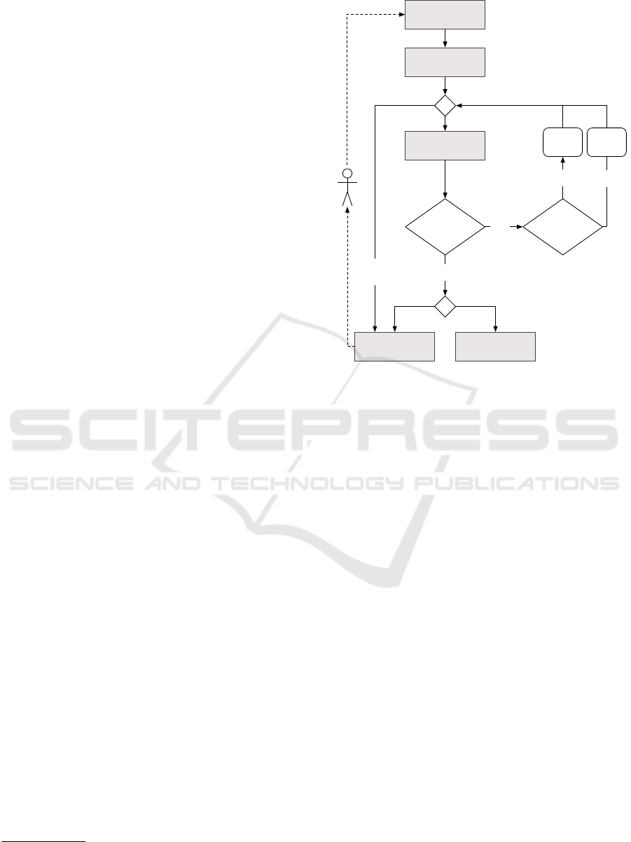
An overview of the working principle is depicted

in Figure 1. Requests are speciﬁed by number of peo-

ple, origin, destination and either pick-up or drop-off

time. Based on the origin and destination, the Request

Processor calculates the shortest path and uses its du-

ration to set the missing time parameter (pick-up or

drop-off). Then, we relax both time constraints by ap-

plying relative and absolute slack times which at the

end give us time windows for both pick-up and drop-

off. The concept of time window (Figure 2) is essen-

tial to increase the overall ﬂexibility of the system.

Without it, the schedules would be too rigid since the

General Transit Feed Speciﬁcation.

https://developers.google.com/transit/gtfs/

Scheduler / Router

Violates

constraints?

Try

again

Request Processor

Bus Sorter

User

Notifier

Bus / Driver

Notifier

Cannot

Yes

Reached

max retries?

Try next

bus

Yes

Figure 1: Working principle overview.

accepted requests would not tolerate to be late or early

as a new request is inserted into the schedule. We ac-

tually model a request as containing two events (pick-

up or drop-off), each of which contains a location, an

actual time and time window.

Afterwards, the Bus Sorter takes over to sort the

buses by their ﬁtness for the new request. Bus Sorter

employs a heuristic with a decision variable. The de-

cision variable is calculated for the new request and

each bus. Then, buses are sorted in descending order

of the decision variables. The original idea in (Tsub-

ouchi et al., 2010) describes only one heuristic: Fa-

voring of the bus that already travels along a direction

to the new request. Additional to that, we implement

multiple strategies for comparison:

1. Prefer idle buses: Distribute the requests in a way,

that the customers are transported faster at the cost

of buses being longer in operation. This heuris-

tic takes sides with the customer (Generally, the

customer and bus service operator have conﬂict-

ing objectives: The customer wants to travel faster

and be earlier at the destination, whereas the bus

service operator wants less buses in service in or-

der to minimize operational costs.).

2. Avoid idling of buses: Prefer buses that are al-

ready in motion/operation, even though it might

prolong the travel time of the customer. This

heuristic takes sides with the operator.

3. Distance: This heuristic considers how far the

Implementation and Evaluation of an On-Demand Bus System

219

EPT

LPT

EDT

LDT

slack time

Available range for IPT

Available range for IDT

time

slack time

Figure 2: Time windows (Tsubouchi et al., 2010). EPT

(LPT): Earliest (latest) pick-up time, EDT (LDT): Earliest

(latest) drop-off time, IPT: Informed pick-up time, IDT: In-

formed drop-off time.

bus would be from the pick-up stop at the de-

sired pick-up time of the new customer, and anal-

ogously from the drop-off stop.

4. Random: Assign random decision variables for

the sake of comparison how the bus sorting strat-

egy inﬂuences the results.

The results are presented in Section 5. The Sched-

uler iterates over the sorted bus list and executes for

each (bus, new request) pair the steps summarized as

follows:

1. Collect all events of the bus.

2. Add 2 events of the new request into collection.

3. Sort the collection of events by actual times.

4. Since the order of events might have changed,

compute new paths between events and update ac-

tual times.

5. Check feasibility of events: If there are violations,

adjust infeasible events. Afterwards, if max re-

tries is not reached, go to Step 3 and try again.

6. Check bus capacity constraint: If there is no vio-

lation, calculate new schedule and return it. Oth-

erwise, if max retries is not reached, go to Step 3

and try again.

If a schedule is returned, we stop iterating over the

remaining buses and conclude that the ﬁtting bus is

found. Overall, the scheduling algorithm aligns with

the one described in (Tsubouchi et al., 2010), but dif-

fers in that, after sorting the events by actual times,

we calculate the paths between successive events and,

if necessary, update actual times (Step 4). This idea

can be illustrated with an example (Figure 3).

Until the insertion of PRE

, the route contains a

path leg PRE

→ PRE

. Since PRE

should be ful-

ﬁlled after PRE

but before PRE

, the vehicle has to

make a detour to pick up the passenger with request

id=5. So there are two new path legs (PRE

→ PRE

and PRE

→ PRE

) that need to be calculated and

PRE

DRE

PRE

DRE

PRE

DRE

Figure 3: Example for insertion of the pick-up request event

(PRE

) and drop-off request event (DRE

) for the request

id=5.

used. This can cause a delay for arrival at PRE

. If

this is the case, then the actual time of PRE

is set

to the newly calculated time (actual time of PRE

plus the duration of PRE

→ PRE

). But now there

might be a conﬂict between PRE

and PRE

, or be-

tween PRE

and its successor, and so on. As it turns

out, the insertion of PRE

can start a chain reaction of

shifting of subsequent events until reaching an event

whose actual time is not affected (i. e. there is a huge

time gap to its predecessor). The insertion of DRE

can cause the same effect and chain reaction.

The potential violation of constraints (e. g. ac-

tual pickup time is later than latest pickup time) are

discovered by applying the feasibility rules and are

solved subsequently (e. g. by setting actual pickup

time to latest pickup time) as described in (Tsubouchi

et al., 2010). If there are no violations for a bus, we

compute the new schedule and notify the user and the

bus driver. If we iterated over all buses but could not

ﬁnd one without violations, we conclude that this re-

quest cannot be accepted.

3.2 Phase 2 - Online Full On-demand

In the second phase, the capabilities of the system

are extended by switching from using a static sta-

tion/connection network to dynamic locations (geo-

coordinates) for pick-up and drop-off. To achieve this,

we need knowledge about the map and road network,

more speciﬁcally a routing solution based on road net-

work.

Moreover, inspired by (Martinez et al., 2006) we

implement a new bus sorting strategy using fuzzy c-

means clustering. Regular k-means, given a distance

function d and a predeﬁned number of k clusters, as-

signs each of n points to one of the k clusters. Instead

of assigning a point to one cluster, fuzzy c-means cal-

culates the membership/likelihood degree of a point

for every cluster. Since we do not choose only one bus

but rather try out all buses, membership/likelihood de-

grees of buses as ﬁtness values allow us to stay within

our framework. This way we can sort clusters (buses)

for a point (route request). Since the already imple-

mented bus sorting strategies were quite primitive,

with this, we wanted to evaluate a more sophisticated

approach whether it would deliver better estimation

for request-bus mapping.

VEHITS 2017 - 3rd International Conference on Vehicle Technology and Intelligent Transport Systems

220

These extensions do not require any modiﬁcation

in Figure 1, only replacing some of the lower level

components with new implementations. The main

component of the system, the scheduler, can be used

as it is. This is the case because it uses the time of

the events as the primary constraint. The space con-

straint (whether we use ﬁxed stations or arbitrary lo-

cations) is only relevant for the underlying routing en-

gine that ﬁnds a path and its duration, which we use to

calculate/set/adjust the times of pick-up and drop-off

events.

4 IMPLEMENTATION

The system is implemented as a standalone Java ap-

plication interacting with PostgreSQL for persistence.

The implementation details speciﬁc to evaluation are

described in Section 5.

In the ﬁrst phase, in which stations are used, the

GTFS data is imported into PostgreSQL once dur-

ing the development using the GTFS SQL Importer

During the initialization, the application fetches the

stations, the arrival/departure times of bus trips at

stations from the database. With this information

we build an undirected graph using JGraphT

. In the

graph, the stations become the nodes and we construct

an edge between two subsequent stations of the same

bus trip. As the edge weight we use the calculated

travel time from a station to the next station in the

same trip. Since we are dependent on the routing be-

tween nodes, JGraphT offers a reliable and fast A*

implementation which we utilize to calculate shortest

paths in the graph. The Bus Sorter component is im-

plemented using the strategy design pattern to make

the exchange of various heuristics easier. The Sched-

uler implementation is the direct translation of the ap-

proach presented in Section 3.1 into Java code.

In the second phase, in order to support routing

between arbitrary locations, we opt for using OTP

OTP is a Java library with an embedded server for efﬁ-

cient pathﬁnding through multi-modal transportation

networks. Transportation networks are represented by

OSM

graph data and optionally extended by GTFS

feeds for transit routes. OTP provides a REST API

for programmatic integration of third-party applica-

tions. The bus system acts as a REST client, and

https://github.com/cbick/gtfs SQL importer

JGraphT is a graph library that provides graph-theory

data models and algorithms. http://jgrapht.org/

OpenTripPlanner. http://www.opentripplanner.org/

OpenStreetMap. http://www.openstreetmap.org/

Representational State Transfer Application Program-

ming Interface

sends routing requests to an OTP instance running lo-

cally. The REST requests specify the transportation

mode as car to trigger pathﬁnding using only the road

network. Fuzzy c-means implementation bases on the

one of Apache Commons Math library

with slight

modiﬁcations for our use case.

5 EVALUATION

In this section, we ﬁrst overview our methodology and

approach how to test the system, as well as the com-

ponents that complement the core implementation to

render such an approach possible. Afterwards, we

present the evaluation results.

5.1 Phase 1 - Online Semi On-demand

The ﬁrst version of the system, which uses existing

bus stations and connections, is evaluated with a sim-

ulation module, that

1. updates the position of the bus as time passes, and

2. generates new requests which are processed by

the system.

It was necessary to simulate the operation of buses

within a short period of time while the service oper-

ation covers a wider range of time. To realize this

we utilize a ticking clock, that is used throughout the

system, to add an offset to the current time when

necessary. Regarding the ﬁrst point, it is checked

whether the bus has arrived at the approaching sta-

tion in schedule. If it is the case, the related entities

are updated (i. e. the schedule, paths, number of pas-

sengers). Regarding the second point, we randomly

generate requests within a bounding box on the map

(which corresponds to service coverage derived from

the GTFS data). In order to achieve a more realistic

simulation, we assign to each station a local density,

that is a function of its distance to all other stations.

It is formulated in Equation (1), where V is the set of

stations in the network and d(u, v) is the direct dis-

tance between u, v ∈ V .

density(v) =

∑

u ∈ V, u 6= v

(d(u, v) + 1)

(1)

The local density is used in Equation (2) to calcu-

late the probability ω of a station to be used as ori-

gin or destination in request generation. With this we

prevent generating excessive number of requests with

stations that in reality are used less frequently.

http://commons.apache.org/proper/commons-

math/userguide/ml.html

Implementation and Evaluation of an On-Demand Bus System

221

ω(v) =

density(v)

∑

u ∈ V

density(u)

(2)

The objective was to run our dynamic system and

simulate a conventional bus service (static system),

send them requests, monitor their status and compare

the results on the basis of following criteria:

Speed denotes how fast the customers arrive at

their destinations. Its value is within the inter-

val [0, 1] ⊂ R. The value of 1 represents the

fastest possible journey from origin to destination,

whereas a value of 0 represents an inﬁnite journey

(in theory). The higher the value, the better.

Capacity Utilization: denotes the average percent-

age of occupied seats during the service time of

a bus. A lower value implies empty trips. The

higher the value, the better.

Success Rate of Requests: expresses the percentage

of accepted requests. The slack time parame-

ter has a huge effect on the success rate, since a

lower slack time infers less ﬂexible time windows,

which inﬂuences the acceptance of new requests

negatively.

Bus Activity: denotes the average percentage of time

during which the buses are in service (motion).

Its value is within the interval [0, 1] ⊂ R. A high

value could imply acceptance of a huge num-

ber of requests, but also an inefﬁcient utilization

of buses (i. e. assignment of a request to a sub-

optimal bus). Therefore it should only be inter-

preted within context of other criteria. Moreover,

this measure only applies to the dynamic system,

since in conventional services the buses are in mo-

tion regardless of the fact that there is demand or

not.

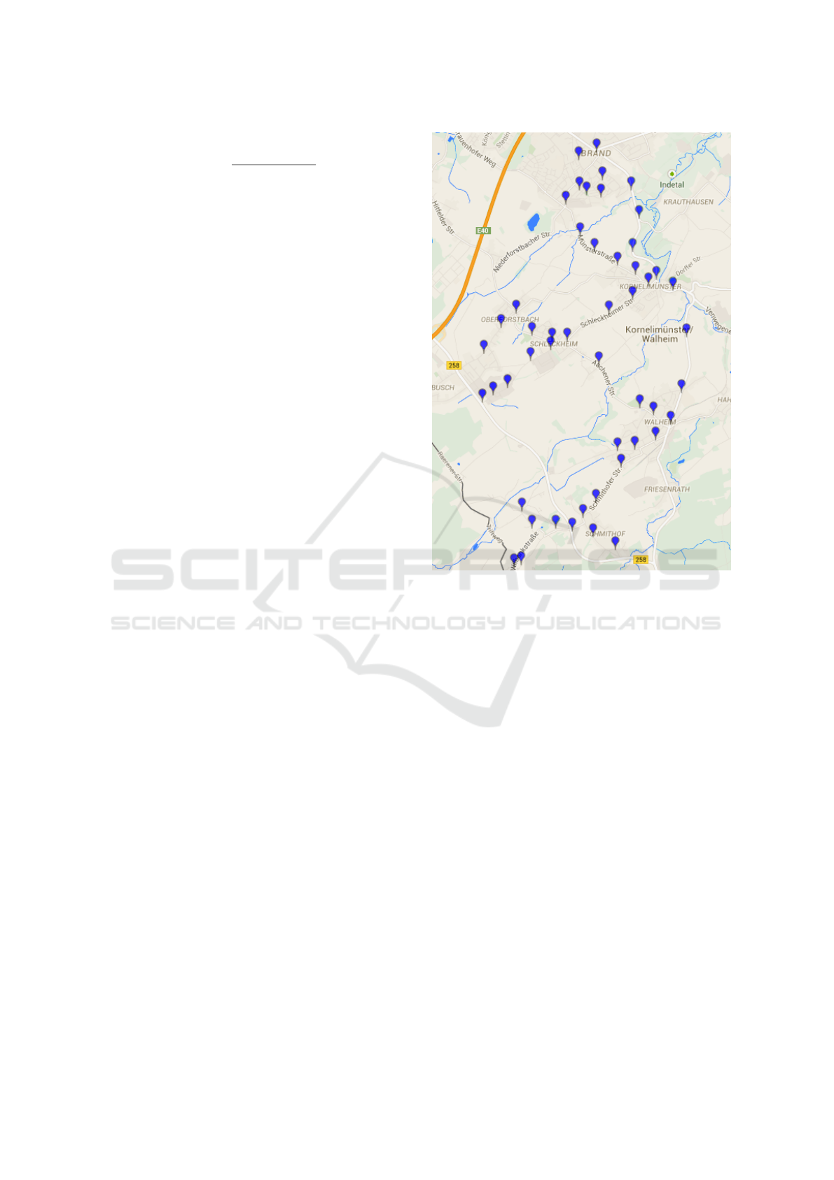
Simulation Conﬁguration. The region used for the

simulation was the south-east rural area of Aachen,

Germany with 52 stations in total (Figure 4). The

simulation of the static system is conﬁgured in a way

that the bus lines as deﬁned in GTFS are used, but

the frequency of a line has to be set. The default bus

line frequency is set to 30 minutes, which corresponds

roughly to the reality in the rural area. In the dynamic

system, the number of buses can be adjusted. More-

over, the relation between the time the request is sent

to the system and the time for requested departure is

important. Journey requests at short notice do not let

the schedule to be adjusted in a timely fashion. There-

fore, the requests must be sent at least 30 minutes and

at most 90 minutes before. In all instances, the sim-

ulation time period is 72 hours. Within this period

approx. 6480 requests are processed (2160 requests

Figure 4: Stations for GTFS in a rural area (south-east of

Aachen, Germany).

per day, 1 request every 40 seconds). Unless stated

otherwise, the absolute slack time is set to 15 minutes

and the relative slack time to 25% of the travel time. It

is also important that both static and dynamic systems

use the same bus capacity which is set to 20.

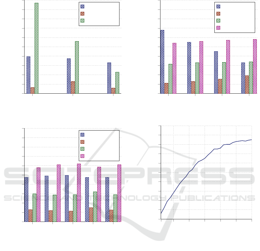
Results. Figure 5 illustrates the effect of different fre-

quencies. This test is conducted to ensure that the

simulation of the static system works as intended.

Success rate decreases as the frequency decreases

(i. e. as the interval between two bus dispatches of the

same bus line increases), which is expected since the

customers are not willing to wait for a longer time.

Figure 6 depicts the results of using different strate-

gies. Interestingly, the results are more or less the

same regardless of the chosen strategy. We argue

that this is due to the chosen, rather small region.

On larger regions this should affect the results pro-

foundly. Figure 7 illustrates the effect of the cho-

sen window size. With increasing time window the

speed decreases, which means it takes longer for the

customers to arrive at the destination, and therefore

the bus capacity utilization increases as well. Fig-

ure 8 aligns with the educated guess ”the more buses

the higher the success rate” but also hints at a satura-

VEHITS 2017 - 3rd International Conference on Vehicle Technology and Intelligent Transport Systems

222

10 20 30

0.1

0.2

0.3

0.4

0.5

0.6

0.7

0.8

0.9

Score

Speed

Capacity util.

Success rate

Figure 5: Static system - Comparison of different frequen-

cies (in min).

Standard

Prefer idle

Avoid idling

Distance

Random

0.1

0.2

0.3

0.4

0.5

0.6

0.7

0.8

0.9

Score

Speed

Capacity util.

Success rate

Bus activity

Figure 6: Dynamic system - Comparison of bus sorting

strategies using 6 buses.

tion point for the maximum number of buses needed

which would be interesting for the operator. Ta-

ble 1 provides a summary of the comparison of the

static/dynamic systems: The static system with 12

buses could only fulﬁll 24% of the requests, whereas

the dynamic counterpart with the same number of

buses can accept 59%. The trips take less time with a

dynamic system as well (67%). Since more requests

are accepted, the dynamic system has a higher capac-

ity utilization (15% compared to 4.5%). In the dy-

namic system, the buses are in motion/service 55% of

the time. During the remaining time they are waiting

idle to service requests. Bus activity calculation of the

static system is omitted, since they are in service all

5 10 15 30

0.1

0.2

0.3

0.4

0.5

0.6

0.7

0.8

0.9

Score

Speed

Capacity util.

Success rate

Bus activity

Figure 7: Dynamic system - Success rate with increasing

time window (in min).

0.1

0.2

0.3

0.4

0.5

0.6

0.7

0.8

0.9

Number of buses

Success rate

Figure 8: Dynamic system - Success rate with increasing

number of buses.

the time during the service operation, which could be

interpreted as 100% bus activity.

5.2 Phase 2 - Online Full On-demand

The second version of the system, now operating with

arbitrary pick-up and drop-off geocoordinates, is eval-

uated by performing quality tests that compare the

request processing of the dynamic and static system

with their results. But ﬁrst, we want to demonstrate

that bus sorting with fuzzy c-means clustering can of-

fer better estimates than prior heuristics.

Bus sorting with fuzzy c-means. In order to evaluate

the clustering strategy, we constructed a test bed with

3 requests (Figure 9). The number of buses was set to

Implementation and Evaluation of an On-Demand Bus System

223

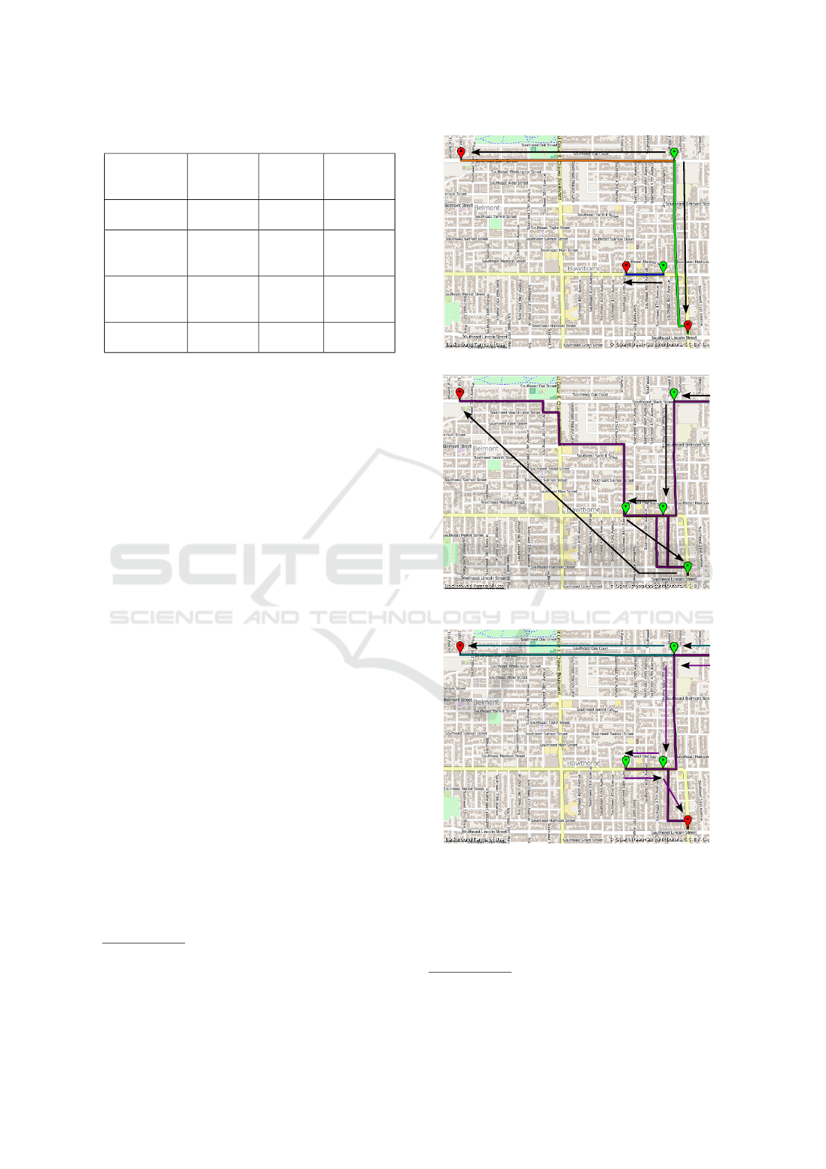
Table 1: Static/dynamic comparison overview.

Static

(12 buses)

Dynamic

(6 buses)

Dynamic

(12 buses)

Success rate

24% 33% 59%

Relative

trip duration

100% 70% 67%

Capacity

utilization

4,5% 15% 15%

Bus activity

– 59% 55%

2, so that the choice of each sorting strategy is easily

visible. Request 1 and 2, color-coded with orange and

green paths respectively, were sent ﬁrst to the system,

specifying the same pick-up time. Figure 10 illus-

trates the resulting bus route of the one bus, to which

all 3 requests were assigned, using the distance strat-

egy (not tested with others since Figure 6 indicated

similar results). This is a viable but sub-optimal bus

route. It causes delays for customers and yields longer

routes for the bus in use. Figure 11 shows the result

using the clustering approach. It employs both buses

(color-coded as green and purple), but the routes of

the buses are shorter and more compact.

Quality Tests

As with the ﬁrst phase of development, we construct

an environment where we run two simulations (dy-

namic and static), generate a request set, let both sys-

tems process the same requests and interpret the out-

come.

Simulation Conﬁguration. The simulation is mod-

eled to mirror the public bus service in Ulm, Germany

operated by Stadtwerke Ulm/Neu-Ulm (SWU). Ulm

is a small to medium-sized city with a comprehensi-

ble transit service. SWU puts its GTFS feed online

which we use for our static system simulation

. We

import the OSM graph of Ulm and the GTFS feed of

SWU into OTP. In REST requests for the dynamic

system the mode parameter is set to car to use only

the OSM graph, and for the static counterpart it is set

to bus to make OTP use the GTFS data. According to

the SWU website, it offers a bus service including 63

buses (with an average capacity of 142), distributed

over 12 bus routes

. The dynamic system is conﬁg-

https://www.swu.de/privatkunden/swu-

nahverkehr/gtfs-daten.html

https://www.swu.de/privatkunden/swu-

nahverkehr/fuhrpark/busse.html

Figure 9: Requests.

Figure 10: Using the distance bus sorting strategy the three

requests are assigned to the same bus.

bus-1 bus-1

bus-2

Figure 11: With fuzzy c-means bus sorting strategy the

three requests are assigned to two buses.

ured in a way to match the static system. The absolute

slack time of the dynamic system was set to 20 min-

utes, which is the average bus frequency calculated

from all bus schedules

. After having looked at the

https://www.swu.de/privatkunden/swu-

nahverkehr/fahrplan-liniennetz/linienfahrplaene.html

VEHITS 2017 - 3rd International Conference on Vehicle Technology and Intelligent Transport Systems

224

GTFS data, we decided to generate requests that fall

in two time periods: From 16:15 to 17:50 and from

21:15 to 22:50. During the ﬁrst time period the static

bus system makes use of all available buses. Within

the second time period only 5 of 11 bus lines are ac-

tive in the static bus system. 5700 requests were gen-

erated for both time periods, which approximates one

request per second. For each time period, the start and

end locations of generated requests fall in one of the

following categories:

1. At bus stations of the same route in static system

2. At bus stations from different routes in static sys-

tem, which means that the customer of the static

system has to switch buses during her journey.

This causes longer travel times and potentially

forces customers to walk a part of their route.

3. Arbitrary locations within the operation bound-

aries independent of any bus route.

This setup presumably should yield results that are in

favor of the static system for the ﬁrst category, and the

dynamic system for the third.

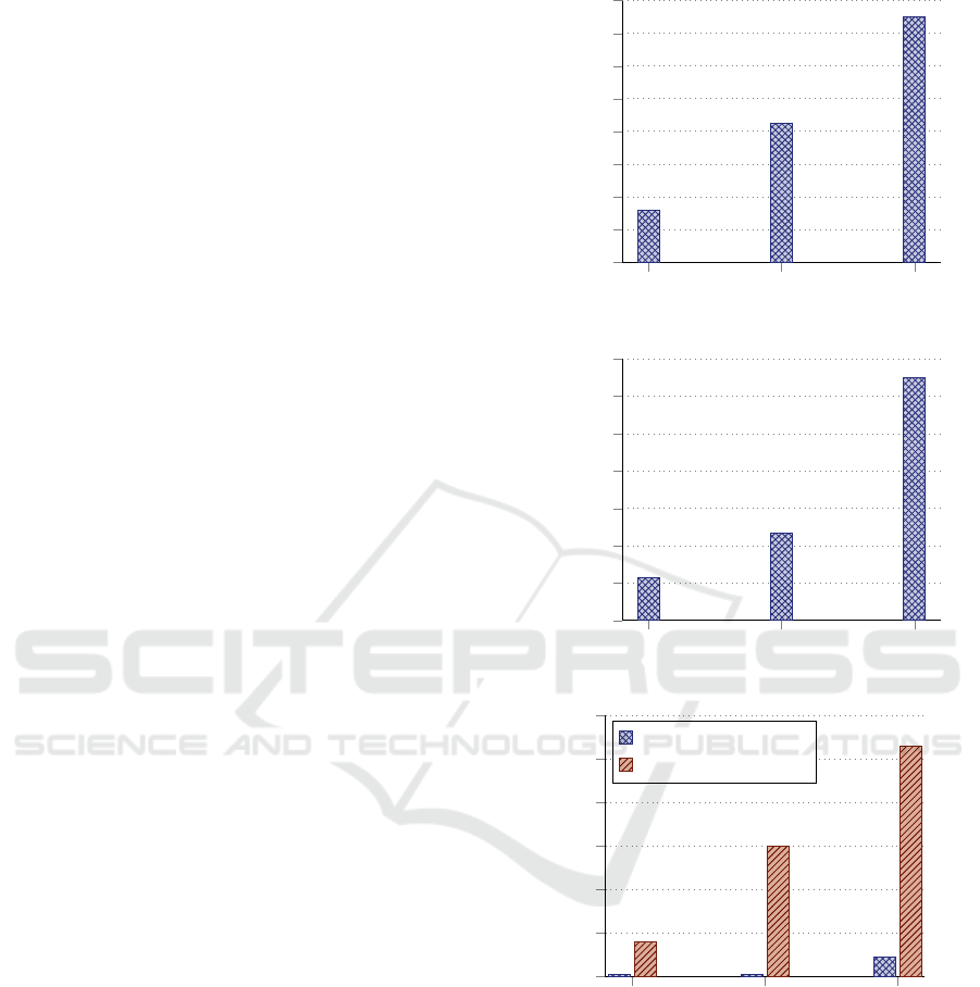
Results. For the sake of brevity we only present the

results of the time period from 16:15 to 17:50. Time

period from 21:15 to 22:50 yielded similar results.

Figure 12 shows the average amount of time the cus-

tomers save using the dynamic system instead of the

static system. In this context, the total travel time

represents the time starting from the desired pick-up

time to the actual drop-off time. This time span thus

includes possible waiting and walking times of cus-

tomers, too. It reveals the tendency of having least

saved time for requests with locations at the same

route, and most saved time for arbitrary request loca-

tions. This matches the expectations since the granted

advantage for the static system decreases with arbi-

trary locations. Moreover, in all cases the amount of

saved time is positive, which shows that customers

have shorter travel times even in scenarios that should

beneﬁt the static bus system. Figure 13 illustrates the

average walking times in the static system since it re-

quires customers to walk to a pick-up station, or be-

tween stations (if there are switches), or from a drop-

off station to their actual destination. In the dynamic

system, there is no such condition. The fact, that the

customers have to walk more for arbitrary locations,

correlates with the expectations. Figure 14 compares

the number of rejections in both systems. The low

number of rejections in the dynamic system can be

explained by having this many buses (63). It almost

always ﬁnds a ﬁtting bus. While the dynamic sys-

tem can by nature reject requests, the rejection for the

static bus system had to be simulated. Therefore, it

was assumed that customers would not wait longer or

Route

Stop Boundary

200

400

600

800

1,000

1,200

1,400

1,600

Average saved time (in s)

Figure 12: Average saved travel time.

Route

Stop Boundary

200

400

600

800

1,000

1,200

1,400

Average walking time (in s)

Figure 13: Average walking time for static system.

Route

Stop Boundary

100

120

1 1

106

Number of rejected requests

On-demand system

Static system

Figure 14: Comparison of rejections.

arrive later than the slack time of the dynamic sys-

tem (20 minutes – average bus frequency). After hav-

ing evaluated both systems using the same conﬁgura-

tion, we wanted to see how much we can scale down

the dynamic system while it still performs at least as

good as the static one. Figure 15 depicts the relation

between the number of buses and the number of re-

jections. So, while the static system has 106 rejec-

tions with 63 buses, the dynamic system can match

the same success rate with 16 buses (107 rejections).

This is valuable for the service provider to cut down

Implementation and Evaluation of an On-Demand Bus System

225

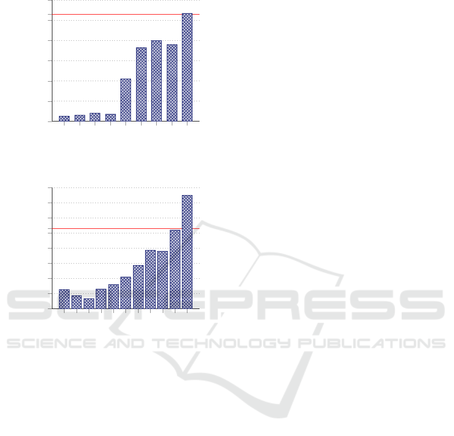
60 50 40 30 20 19 18 17 16

100

120

Number of buses

Number of rejected requests

Figure 15: Optimal number of buses. The horizontal line

represents 106 rejections of the static system with 63 buses.

20 19 18 17 16 15 14 13 12 11 10

100

120

140

160

Slack time (in min)

Number of rejected requests

Figure 16: Optimal slack time for 30 buses. The horizontal

line represents 106 rejections of the static system with 63

buses.

operational costs. Next, we wanted to see how much

we can reduce the slack time. A broader slack time

provides the needed ﬂexibility to our dynamic sys-

tem, but is inconvenient for the customer. Figure 16

shows that we can reduce the slack time to 11 min-

utes with 30 buses and match the success rate of the

static system (63 buses with 20 minutes average bus

frequency).

6 CONCLUSION

In this work, we implemented and evaluated an online

full on-demand bus system in two phases. We started

with a preliminary version that routes freely from sta-

tion to station, but visits only the stations where cus-

tomers are to be picked up or dropped off. This al-

lowed us to evaluate the feasibility of an on-demand

system before advancing the approach. We evaluated

it in comparison with a traditional bus service simu-

lation using a rural area (south-east of Aachen, Ger-

many), where the quality of bus services usually suf-

fer from low density of bus stations and low bus fre-

quencies. The comparison was done on the basis of

efﬁciency criteria such as speed, capacity utilization,

success rate and bus activity. The evaluation showed

that the dynamic system can deliver better results with

the same (or less) number of buses as in the static sys-

tem.

In the second phase, we extended the system to

route between arbitrary locations and replaced the

bus sorting strategy with a more sophisticated one.

The tests showed that the new bus sorting approach

yielded a better order of buses for the to-be-processed

request. Furthermore, comparisons were performed

with the static counterpart by running simulations

within an urban region (as opposed to a rural area

of the ﬁrst phase), namely the transit service area of

Ulm, Germany. These demonstrated clear advantages

in terms of saved travel time, non-existing walking

time and number of accepted requests when using the

same conﬁguration as in the static system. We also

determined that the dynamic system requires less re-

sources in order to provide the same quality of service

of the static system.

Future Work

This work presented the basic approach, implemen-

tation and evaluation. It serves as a basis for further

experimentation and improvements.

The evaluation methodology takes priority in the

list of planned improvements. Even though the com-

parison of a new solution (on-demand bus system) to

an existing solution (traditional bus service) is valu-

able, its realization is crucial for the end result. In

particular, we need better insight and more statisti-

cal data about the bus service or the usage/travel pat-

terns of customers for the evaluated area. Simulat-

ing a traditional static bus system or generating cus-

tomer requests might not represent the reality. In or-

der to improve request generation we plan to utilize

agent-based modeling. We also would like to conduct

ﬁeld tests in order to evaluate the system, but also to

validate the simulation results. Another aspect, the

request-processing performance of the system, is not

considered so far and is part of the future work.

Then there are features that we want to imple-

ment to enhance the capabilities of the system. In the

current implementation, the bus picks up and drops

off customers precisely at the given locations with no

ﬂexibility in this regard. But in a real setting, these

locations might be very close to each other and still

force the bus to stop for every single customer which

VEHITS 2017 - 3rd International Conference on Vehicle Technology and Intelligent Transport Systems

226

would not be desirable due to caused trafﬁc conges-

tion or bad user experience of customers within the

bus. To overcome this, assembly points could be

derived, where customers close to each other (e. g.

within a radius) can meet before the bus picks them

up, or multiple customers can be dropped off at the

same location if their desired locations are close to

each other. This brings us to the next feature of in-

corporating user preferences. The radius for assem-

bly points can be set system-wide and identical for

every customer, which would not be desirable. In

the same light, the slack time for the requests is cur-

rently set system-wide and identical for every cus-

tomer. Customers should be able to provide their own

preferences, which are used in the request processing

pipeline. This is also part of future work.

ACKNOWLEDGMENTS

This work was partially funded by German Federal

Ministry of Economic Affairs and Energy (BMWi)

for the project Mobility Broker (01ME12136) as well

as for the project Digitalisierte Mobilit

at – Die Offene

Mobilit

atsplattform (DiMo-OMP).

REFERENCES

Amoroso, S., Migliore, M., Catalano, M., and Galatioto,

F. (2010). A demand-based methodology for planning

the bus network of a small or medium town. European

Transport / Trasporti Europei, 44:41–56.

Beutel, M. C., G

okay, S., Kluth, W., Krempels, K.-H.,

Ohler, F., Samsel, C., Terwelp, C., and Wiederhold,

M. (2016). Information Integration for Advanced

Travel Information Systems. Journal of Trafﬁc and

Transportation Engineering, 4:177–185.

Beutel, M. C., G

okay, S., Kluth, W., Krempels, K.-H., Sam-

sel, C., and Terwelp, C. (2014). Product oriented in-

tegration of heterogeneous mobility services. In 17th

International IEEE Conference on Intelligent Trans-

portation Systems (ITSC), pages 1529–1534.

Cordeau, J.-F. and Laporte, G. (2007). The dial-a-ride prob-

lem: models and algorithms. Annals of Operations

Research, 153(1):29–46.

Crainic, T. G., Errico, F., Malucelli, F., and Nonato, M.

(2010). Designing the master schedule for demand-

adaptive transit systems. Annals of Operations Re-

search, 194(1):151–166.

Desaulniers, G., Desrosiers, J., Erdmann, A., Solomon,

M. M., and Soumis, F. (2001). The Vehicle Routing

Problem. In Toth, P. and Vigo, D., editors, The Ve-

hicle Routing Problem, chapter VRP with Pickup and

Delivery, pages 225–242. Society for Industrial and

Applied Mathematics, Philadelphia, PA, USA.

El-Sherbeny, N. A. (2010). Vehicle routing with time win-

dows: An overview of exact, heuristic and metaheuris-

tic methods. Journal of King Saud University - Sci-

ence, 22(3):123–131.

Gørtz, I. L. (2006). Hardness of preemptive ﬁnite capac-

ity dial-a-ride. In in Computer Science, L. N., edi-

tor, Proceedings of 9th International Workshop on Ap-

proximation Algorithms for Combinatorial Optimiza-

tion Problems (APPROX 2006).

Kluth, W., Beutel, M. C., G

okay, S., Krempels, K.-H., Sam-

sel, C., and Terwelp, C. (2015). IXSI - Interface for

X-Sharing Information. In 11th International Confer-

ence on Web Information Systems and Technologies.

Li, Y., Wang, J., Chen, J., and Cassidy, M. J. (2007). De-

sign of a demand-responsive transit system. Califor-

nia PATH Program, Institute of Transportation Stud-

ies, University of California at Berkeley.

Martinez, M. V., Simari, G. I., Castillo, C. D., and Peer,

N. J. (2006). A GPS-Based On-Demand Shuttle Bus

System. Technical report, Department of Computer

Science, University of Maryland College Park.

Mukai, N. and Watanabe, T. (2005). Dynamic Transport

Services Using Flexible Positioning of Bus Stations.

Autonomous Decentralized Systems, pages 259–266.

Ronald, N., Thompson, R., Haasz, J., and Winter, S. (2013).

Determining the viability of a demand-responsive

transport system under varying demand scenarios. In

Proceedings of the Sixth ACM SIGSPATIAL Inter-

national Workshop on Computational Transportation

Science, IWCTS ’13, pages 7:7–7:12, New York, NY,

USA. ACM.

Savelsbergh, M. W. P. and Sol, M. (1995). The General

Pickup and Delivery Problem. Transportation Sci-

ence, 29:17–29.

Tsubouchi, K., Yamato, H., and Hiekata, K. (2010). Inno-

vative on-demand bus system in Japan. IET Intelligent

Transport Systems, 4(4):270–279.

Implementation and Evaluation of an On-Demand Bus System

227