
Linear Photometric Stereo using Close Lighting Images
based on Intensity Differential
Zennichiro Sasaki, Fumihiko Sakaue and Jun Sato
Nagoya Institute of Technology, Nagoya, Japan
{sasaki@cv., sakaue@, junsato@}nitech.ac.jp
Keywords:
Photometric Stereo, Surface Normal Reconstruction, Close Light Source.
Abstract:
In this paper, we propose a new linear photometric stereo method from images taken under close light sources.
When an images are taken under close light source, we can obtain not only surface normal but also shape
from the images. However, relationship between observed intensity and object shape is not linear, and then,
we have to use non-linear optimization to estimate object shape. In order to estimate object shape by just
linear estimation, we focus not only direct observed intensities, but also differentials of the intensities in this
paper. By using the set of observed intensity and its differentials, we can represent relationship between object
shape and intensities linearly. By this linear representation, linear estimation of object shape achieved even
if obtained images are taken under close light sources. Experimental results show our proposed method can
reconstruct object shape by only linear estimation efficiently and accurately.
1 INTRODUCTION
Object shape reconstruction from camera images is
one of the most important problem in field of com-
puter vision. Especially, shape reconstruction taken
under different lighting environment, so called pho-
tometric stereo(Woodham, 1980), is useful for apply-
ing to research on Computer Graphics (CG) and Vir-
tual Reality (VR) since the method can directly recon-
struct surface normal which is important for rendering
image. Therefore, this kind of methods are widely
studied and practically used(Chen et al., 2011; Bros-
tow et al., 2011) recently.
In the traditional photometric stereo method, there
are two strong assumptions. The first assumption is
related to reflection and it assumed that reflection on
the object surface can be described by Lambert (dif-
fuse) reflection model. The second assumption is
for light sources and it assumed that a light source
is placed on infinite point in the scene. In order to
relax these assumptions, many kinds of methods are
proposed. However, effect of first assumption relax-
ation is limited since most of the object surface can
be approximately represented by Lambert model. Of
course although specular reflection such as hi-light
cannot be represented by this model, effect of them
is in limited case. For example, specular reflection by
Phong model can be observed only when a viewpoint
is on specular direction of a light source. That is, this
kind of reflection cannot be observed from most of the
viewpoints.
On the other hand, set up of light source by sec-
ond assumption includes serious problem. If light
source is placed at not infinite point but close to the
object, light source direction of each point on the sur-
face changes drastically. In this case, surface normal
cannot be estimated correctly. Therefore, we have to
maintain large space to utilize photometric stereo. In
order to avoid this problem, several methods which
use a close point light source are proposed(Iwahori,
1990; Kim and Burger, 1991; Okabe and Sato, 2006;
Hayakawa, 1994). In these methods, distance be-
tween the point light source and the target object is
near, and then, it is not necessary to prepare a large
space. Furthermore, these methods can obtain addi-
tional information which is lost in images taken under
an infinite point light source. That is, these images in-
clude not only surface normal information, but also
object shape information. Therefore, object shape
can be reconstructed directly by the methods. How-
ever, since relationship between observed intensities
and object shape is non-linear, these methods require
non-linear optimization which requires large compu-
tational cost.
In order to avoid this problem, linear shape esti-
mation methods are proposed(Fujita et al., 2009; Kato
et al., 2010). Although these methods can reconstruct
object shape and surface normal by only linear esti-
Sasaki Z., Sakaue F. and Sato J.
Linear Photometric Stereo using Close Lighting Images based on Intensity Differential.
DOI: 10.5220/0006265506230630
In Proceedings of the 12th International Joint Conference on Computer Vision, Imaging and Computer Graphics Theory and Applications (VISIGRAPP 2017), pages 623-630
ISBN: 978-989-758-225-7
Copyright
c
2017 by SCITEPRESS – Science and Technology Publications, Lda. All rights reserved
623
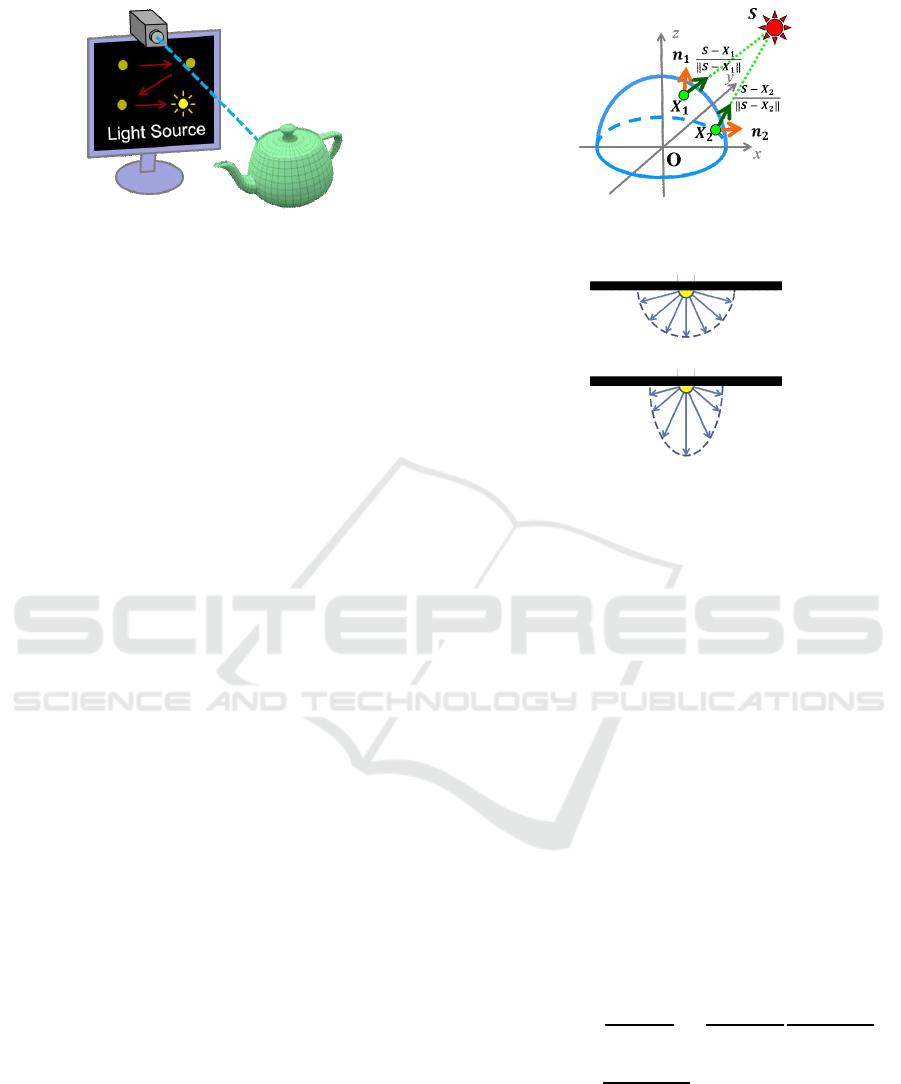
Figure 1: Video display device as a set of light sources. By
using the display, position of light source can be controlled
easily and quickly.
mation, they used approximated intensity model, and
then, accuracy of these methods are not better. There-
fore, more accurate linear representation is required
for effective object shape estimation. In this paper,
we propose a new linear shape reconstruction method
using images taken under close light source without
any approximation. For this objective, we focus not
only observed images, but also differentials of the ob-
served images. In addition, we propose a compact
shape estimation system based on the proposed shape
reconstruction method. In this system, we use a video
display as a set of light sources as shown in Fig.1. By
using the display, position of light source can be con-
trolled easily and quickly. In order to use the system
we need to describe intensity model including light-
ing characteristic of the display since this character-
istics depends on products. By using our proposed
method and this system, we measure the object shape
efficiently and accurately.
2 INTENSITY OBSERVATION
MODEL
2.1 Lambert Model
We first describe intensity observation model on sur-
face of objects. We, in this paper, assume that re-
flectance property of the surface can be described by
Lambert model. Let s and n denote light source di-
rection and surface normal direction, respectively. In
this case, the observed intensity I can be represented
as follows:
I = max(Eρn
⊤
s,0) (1)
where E is powerof the light source and ρ is albedo of
the surface. When there is no shadow on the surface,
the Eq.(1) can be rewritten as follows:
I = Eρn
⊤
s. (2)
The equation indicates that the normal direction n can
be linearly estimated from a set of intensity and a set
Figure 2: Relationship among a light source position S, 3D
point X on an object surface and surface normal n.
(a) Ideal light source
(b) Ordinary light source
Figure 3: Light source characteristics: a light source (a)
emit light rays to all direction constantly. Power of light
rays from a light source (b) changes by directions of light
rays.
of s. This is traditional surface normal estimation by
a photometric stereo method(Woodham, 1980).
2.2 Under Close Light Source
We next consider the case when a light source is close
to the object surface. In this case, light source direc-
tion s is different from each other on the surface point
X as shown in Fig.2. In addition, we need to con-
sider light source characteristics since power of light
ray from the light source changes by direction in or-
dinary case as shown in Fig.3. Especially, we use a
video display device as a light source, and then, we
need to consider this characteristics carefully. There-
fore, intensity observation model cannot be simply
described like Eq.(2). In this paper, we define the in-
tensity model as follows:
I
c
= E
S− X
||S− X||
ρ
1
||S− X||
2
n
⊤
(S− X)
||S− X||
= E
d
ρ
n
⊤
(S− X)
||S− X||
3
(3)
where S is a position of the light source and X is a 3D
point on the surface. A function E represents charac-
teristics of light. Output of this function is changed
by light ray direction d = (S− X)/||S− X||. To sim-
plify description, the function E ((S − X)/ ||S− X||)
is written by E
d
.
VISAPP 2017 - International Conference on Computer Vision Theory and Applications
624

In this equation, a denominator of first component,
i.e. ||S − X||
2
, indicates attenuation of the light by
distance. Although the attenuation can be ignored in
Eq.(2) because distance from a light source is suffi-
ciently far, we need to consider the effect of atten-
uation in our model. In addition, light source char-
acteristic E
d
should be considered by the same rea-
son. Considering of these components, this intensity
model become non-linear, and then, non-linear opti-
mization must be used to estimate surface normal and
object shape from a set of intensities.
3 LINEAR SURFACE
ESTIMATION USING
INTENSITY DIFFERENTIALS
3.1 Intensity Differential based on
Observation
In order to deal with close lighting images more eas-
ily, we focus on not only direct observed intensity by
Eq.(3), but also differentials of the observed intensi-
ties.
One of the main factor of non-linearity in Eq.(3)
is normalization of lighting direction (S−X) by ||S−
X||. In order to avoid this explicit normalization, in-
tensity approximation(Fujita et al., 2009) model is
proposed. Although this model achieves simplifying
of the equations, accuracy of the method is not high
because of the approximation. In this paper, we do
not use any approximation for describing the intensi-
ties. For this objective, we focus on differentials of
intensities with respect to light source positions. By
using the differentials, we can simplify description of
intensity without any approximation.
Before explanation of our proposed model, we
briefly mention measurement of intensity differentials
in our system. Let I(S
1
) and I(S
1
+ ∆S) denote inten-
sities taken under a light source arranged at S
1
and
S
1
+ ∆x(= [∆x,0, 0]
⊤
). Differentials of the intensity
can be described by difference of them, and then, ap-
proximated differential I
x
(S) can be computed as fol-
lows:
I
x
(S) ∼
I(S+ ∆x) − I(S)
∆x
(4)
As same as this manner, I
y
(S) can be computed as
follows:
I
y
(S) ∼
I(S+ ∆y) − I(S)
∆y
(5)
In fact, these equation indicates that we need to obtain
more number of images for estimating differentials.
However, it is not serious problem in our system. In
our system, a video display device is used as a set of
light sources, and then, the light source can be moved
flexibly and quickly. Therefore, we can measure dif-
ferentials of intensity quickly.
Note that we cannot measure differential of inten-
sity wrt s
z
in our system since a light sources can be
moved only on the display plane.
3.2 Linear Representation of Intensity
and Differentials
Let us consider differentials of intensities with re-
spect to light source positions theoretically. We first
consider the case when light ray characteristics are
constant, that is, E(d) = E. Under this assumption,
Eq.(3) can be simply rewritten as follows:
I = Eρ
n
⊤
(S− X)
||S− X||
3
(6)
Differentiatingof Eq.(6), differentialsI
x
and I
y
respect
to s
x
and s
y
can be described as follows:
I
x
= Eρ
n
x
||S− X||
2
− 3n
⊤
(S− X)(s
x
− x)
||S− X||
5
(7)
I
y
= Eρ
n
y
||S− X||
2
− 3n
⊤
(S− X)(s
y
− y)
||S− X||
5
(8)
In addition, we rewritten Eq.(6) as follows:
I = Eρ
n
⊤
(S− X)||S− X||
2
||S− X||
5
(9)
In these equations, denominators of all equation are
the same. Therefore, these equation can be rewritten
by using homogeneous representation as follows:
λ
I
x
I
y
I
=
n
x
||S− X||
2
− 3n
⊤
(S− X)(s
x
− x)
n
y
||S− X||
2
− 3n
⊤
(S− X)(s
y
− y)
n
⊤
(S− X)||S− X||
2
(10)
In this equation, denominators ||S−X||
5
, light source
energy E and reflectance ρ are eliminated since homo-
geneous representation allows scale ambiguity. These
components are included in all equations, and then,
they are written by just λ. By this simplification, com-
plicated component ||S− X||
5
can be ignored in this
model.
3.3 Linear Intensity Representation by
Light Projection Matrix
We next expand these equations for linear intensity
representation. In this expansion, we use constraint
with s
z
for simplifying the equations. In the previous
section, we mentioned that a set of light sources are
Linear Photometric Stereo using Close Lighting Images based on Intensity Differential
625

on a display plane. The fact indicates that s
z
can be
constant in the intensity representation. In this paper,
we define that s
z
= 0 and we expand intensity repre-
sentation by using this definition.
We expand Eq.(10) and separate it into two matri-
ces. A first matrix is a 3× 8 matrix P based on object
shape X and surface normal n. This matrix P is de-
scribed as follows:
P =
0 0 −2n
x
n
x
0 0 n
y
−2n
y
n
x
n
y
−(n
⊤
X+ 2n
y
y) −(n
⊤
X+ 2n
y
y)
−3n
y
3n
⊤
X− n
x
x
−3n
x
−2n
y
x+3n
x
y
−2(n
y
x+n
x
y) n
x
X
⊤
X+ 2xn
⊤
X
3n
y
x−3n
x
y n
x
X
⊤
X− 3xnn
⊤
X
3n
⊤
X+ n
y
y n
t
X
⊤
X− 3yn
⊤
X
n
y
X
⊤
X+ 2yn
⊤
X n
⊤
XX
⊤
X
(11)
The next component is an 8-dimensional vector L
based on light source position S and it is described
as follows:
L=
s
5
x
+ s
x
s
2
y
s
3
y
+ s
2
x
s
y
s
2
x
s
2
y
s
x
s
y
s
x
s
y
1
⊤
(12)
By using P and L, set of intensity [I,I
x
,I
′
y
]
⊤
can be
represented linearly as follows:
λ
I
I
x
I
y
I = PL (13)
By using this representation, we can describe changes
of intensity depends on position of a light source lin-
early. In this paper, P and L are called light projection
matrix and light information vector respectively.
3.4 Linear Shape Estimation
We next consider linear estimation of object shape. In
fact, light projection matrices include object shape X
and surface normal n directly, and then, the compo-
nents can be computed easily when the light projec-
tion matrix can be estimated. Therefore, we explain
estimation method of the matrix P.
Let L
i
and I
i
denote a light information vector
and observed intensities under i-th (i = 1, ··· , N) light
source position. In this case, Eq. (13) can be rewritten
as follows:
λ
i
I
i
= PL
i
(14)
where λ
i
is a scale ambiguity. For eliminating this
ambiguity, we transform the equation by using skew
symmetric matrix [I]
×
as follows:
[I
i
]
×
I
i
= λ
i
[I
i
]
×
PL
i
= 0 (15)
When λ
i
is not 0, the λ
i
can be eliminated by dividing
by itself. Therefore, we can obtain linear constraint
from N images as follows:
L
⊤
1
[I
1
]
×
.
.
.
L
⊤
N
[I
N
]
×
P
⊤
= 0 (16)
By solving this equations, the light projection matrix
P can be estimated. This solution can be provided by
ordinaryleast means square method since they are just
linear equations. That is, linear estimation of object
shape is achieved without any approximation.
4 INTENSITY REPRESENTATION
WITH LIGHT SOURCE
CHARACTERISTICS
4.1 Intensity Differential with
Characteristic
In this section, we consider linear intensity represen-
tation with light source characteristics. In this case,
light source energy E in all equations are replaced
to light source characteristics E
d
. The characteris-
tic function E
d
depends on S, and then, E
d
changes
by changing of S. Therefore, we need to reflect this
effect to differentials of intensities.
In fact, this reflection is not so difficult since E
d
is just multiplier. By using observed intensity I and
power of light E in Eq.(6), observed intensity I
′
which
includes characteristics E
d
can be described as fol-
lows:
I
′
= E
d
ρ
n
⊤
(S− X)||S− X||
2
||S− X||
5
= E
d
I
E
(17)
As same as this manner, differentials I
′
x
and I
′
y
can be
described by I
x
and I
y
as follows:
I
′
x
= E
d
I
x
E
+ E
d
x
I
E
(18)
I
′
y
= E
d
I
y
E
+ E
d
y
I
E
(19)
where E
d
x
and E
d
y
are differentials of light source
characteristic with respect to s
x
and s
y
respectively.
Therefore, observed set of intensities I
′
including E
d
can be described as follows:
I
′
=
1
E
E
d
0 E
d
x
0 E
d
E
d
y
0 0 E
d
I
x
I
y
I
= E
d
PL (20)
where E includes light source characteristics and its
differentials. By using this equations, images taken
under close light source can be described linearly
even if light source characteristic is not constant.
VISAPP 2017 - International Conference on Computer Vision Theory and Applications
626
4.2 Shape Estimation with
Characteristic
We next consider shape reconstruction by Eq.(20). At
glance, light projection matrix P can be estimated by
the same way to Eq.(16) which does not include E.
However, we cannot utilize this method because E
depends on not only light source position S, but also
reconstructed shape X. Therefore, we use iterative es-
timation method for estimating a projection matrix P.
In this iterative method, we first provide initial
light source direction d = [0, 0,1]
⊤
for each point.
From the initial direction, E
0
can be computed di-
rectly. When E
0
is obtained from it, we can estimate
P linearly under the characteristics as follows:
L
⊤
1
[E
−1
0
I
1
]
×
.
.
.
L
⊤
N
[E
−1
0
I
N
]
×
P
⊤
0
= 0 (21)
From this equation, object shape X
0
based on P
0
can
be estimated, and then, a direction d
0
can be updated
to d
1
as follows:
d
1
=
S− X
0
||S− X
0
||
(22)
From this updated direction, E
0
can be also updated to
E
1
. Therefore, a projection matrix P
i
for i-th iteration
can be estimated as follows:
L
⊤
1
[E
−1
i
I
1
]
×
.
.
.
L
⊤
N
[E
−1
i
I
N
]
×
P
⊤
i
= 0
We finally obtain appropriate shape X and surface
normal n based on matrix P.
Note that, we can obtain not only surface normal
n, but also object shape X from the estimated projec-
tion matrix P. However, accuracy of estimated X is
not better since effect of surface normal n is stronger
than effect of X in observed intensities. Therefore, we
have to combine these two estimated result for more
accurate estimation. In this combining, surface nor-
mal n is integrated to object shape around estimated
shape X. By using direct shape estimation result X in
this integration, we can reconstruct object shape even
if the object includes discontinuous surface. By us-
ing both two components, our method can reconstruct
object shape accurately and stably.
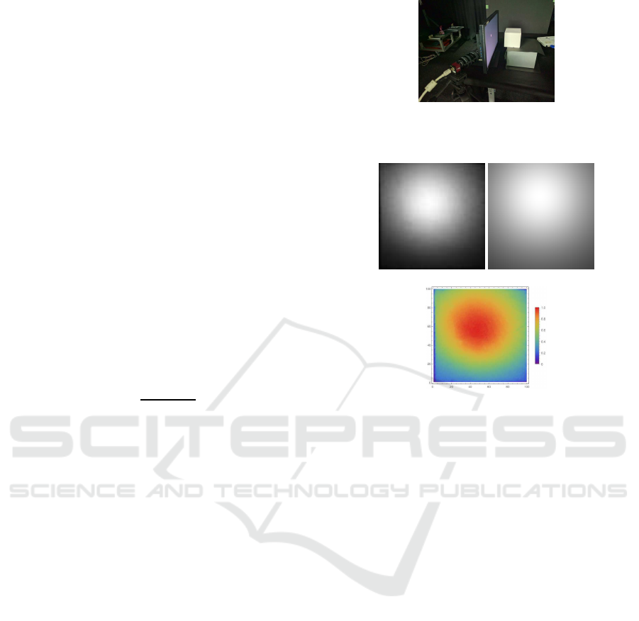
Figure 4: Display characteristics measurement: light source
on the display moved, and changes of intensities on the cube
were measured.
(a) measured image (b) synthesized image
(c) measured
characteristics
Figure 5: Three images for measuring light source char-
acteristic: (a) is measured image, (b) is synthesized image
taken under ideas light source and (c) is estimated E from
(a) and (b).
5 EXPERIMENTAL RESULTS
5.1 Measurement of Light Source
Characteristics
Let us show some experimental result by our pro-
posed method. We first show measurement result of
display (light source) characteristics for validating our
proposed intensity model by Eq.(3). In this measure-
ment, we set up a display device and a plaster cube
which had Lambert surface as shown in Fig.4. A light
source on the display was moved and images were
taken under each light source position. An example of
taken image is shown in Fig.5(a). For estimating E
d
,
distance between the display and the light source was
measured directly, and an image taken under ideal
(constant) light source characteristics was synthesized
as shown in Fig.5(b) by Eq.(6). From these images,
light source characteristics E
d
of each pixel was es-
timated as shown in Fig.5(c). By integration of esti-
mated E
d
taken under different light source position,
the whole characteristic E
d
is estimated. The esti-
Linear Photometric Stereo using Close Lighting Images based on Intensity Differential
627
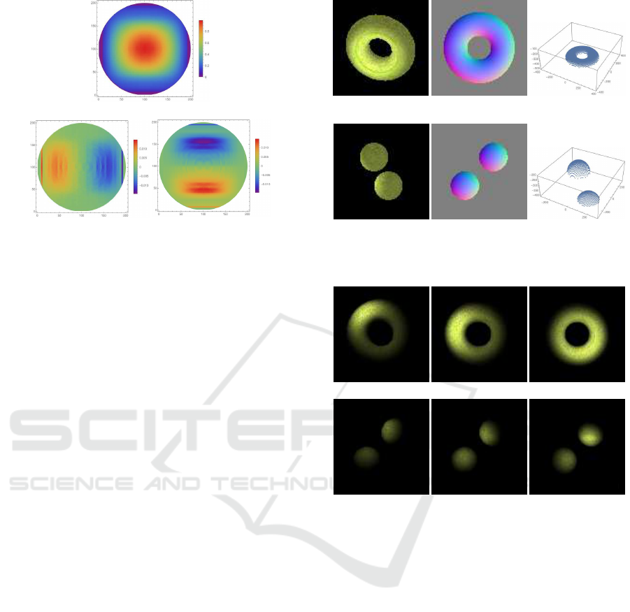
(a) Light source characteristic
(b) Differential E
x
(c) Differential E
y
Figure 6: Measured light source characteristics:(a) shows
direct characteristic E and (b),(c) show differentials E
x
and
E
y
respectively.
mated result is shown in Fig.6(a) and differentials E
x
and E
y
is also shown in Fig6(b) and (c). In these fig-
ures, a direction vector d is parallel projected onto
xy-plane, i.e. E ([d
x
,d
y
,d
z
]
⊤
) is represented at a point
(d
x
,d
y
). These results indicate that characteristics of
the provided display is not constant obviously. That
fact indicates Eq.(9) is not sufficient to represent ob-
served intensities taken under the display. Therefore,
we need to utilize Eq.(3) to represent intensities and
estimate object shape accurately.
5.2 Environment
We next show shape reconstruction result by using
our proposed method. We describe experimental en-
vironment at first. In this experiment, we constructed
experimental environment in computers and synthe-
sized images in this simulation environment. Figure7
shows target objects for shape reconstruction. The
target (b) includes discontinuous surface which can-
not be differentiated. These objects are illuminated
by a display in the scene. Light source characteris-
tics measured in 5.1 was utilized for characteristics
of this display. By using the display illumination, in-
put images were synthesized under 100 different light
source positions. Several examples of the images are
shown in Fig.8. From these images, differentials of
intensity were computed and object shape was recon-
structed by our proposed method. For comparison,
object shape was also reconstructed by an traditional
photometric stereo method. In this method, surface
normal were reconstructed under infinite light source
assumption and shape was estimated by integration of
the surface normal.
(i) object (ii) surface normal (iii) object shape
(a) Torus
(i) object (ii) surface normal (iii) object shape
(b) Two balls
Figure 7: Target objects: (a) Torus and (b) two balls.
(a) Torus
(b) Two balls
Figure 8: Examples of synthesized images.
5.3 Results
Reconstructed results of a torus are shown in Fig.9.
In this figure, reconstructed surface normal and re-
constructed shape are compared to a result by an tra-
ditional photometric stereo method. These figure in-
dicates that although surface normal can be estimated
by our proposed method, it cannot be reconstructed by
the traditional method because the method cannotrep-
resent changes of light source direction, light source
characteristics, and intensity attenuation by distance
accurately. In shape reconstruction result, although
direct estimation result shown in Fig.9(v) is not so ac-
curate, the accuracy can be improved drastically by
combining surface normal estimation result and ob-
ject shape reconstruction result as shown in Fig.9(vi).
This is because the accuracy of surface normal es-
timation is higher than object shape estimation. On
the other hand, reconstructed shape by the traditional
method is not accurate since surface normal cannot be
VISAPP 2017 - International Conference on Computer Vision Theory and Applications
628
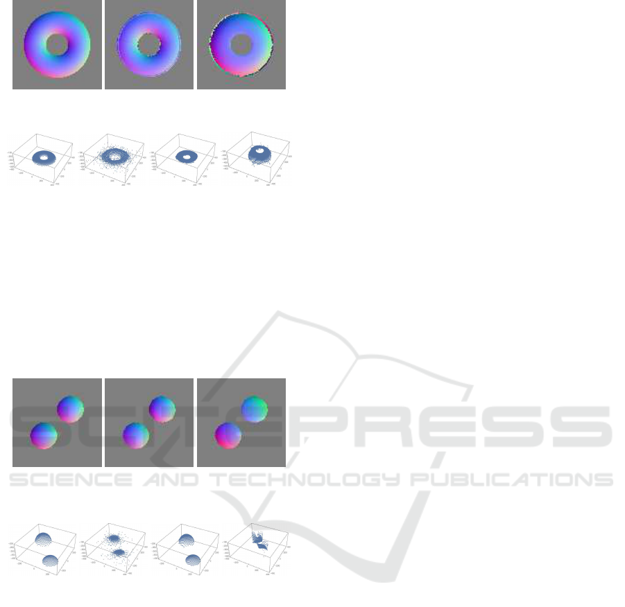
(i) ground truth of
surface normal
(ii) surface normal
by proposed
method
(iii) surface normal
by traditional
method
(iv) ground
truth of object
shape
(v) direct
estimated
shape by
proposed
method.
(vi) estimated
shape from X
and n by
proposed
method
(vii) estimated
shape by
traditional
method
Figure 9: Reconstructed result of torus: (i), (ii) and (iii)
show (i) ground truth of surface normal, (ii)estimated re-
sult by our proposed method and (iii)estimated result by
traditional method. (iv)∼(vii) show (iv)ground truth of
object shape, (v)direct estimated shape from P by our
method, (vi) final reconstructed shape using n and X and
(vii)reconstructed shape by traditional method.
(i) ground truth of
surface normal
(ii) surface normal
by proposed
method
(iii) surface
normal by
traditional
method
(iv) ground
truth of object
shape
(v) direct
estimated
shape by
proposed
method.
(vi) estimated
shape from X
and n by
proposed
method
(vii) estimated
shape by
traditional
method
Figure 10: Reconstructed result of two balls.
estimated accurately with their assumptions.
Figure 10 shows estimated results of two balls. In
this result, although our method can reconstruct sur-
face normal and object shape accurately, the tradi-
tional method cannot reconstruct them. Especially, as
shown in Fig.10(vi), shape of the two balls can be es-
timated validly by our method even if two balls have
different depth from each other. In our method, direct
shape estimation results and integrated surface normal
are combined for estimating object shape, and then,
discontinuous surface can be reconstructed correctly.
These results indicate that our method can reconstruct
object shape and surface normal accurately. That is,
our linear intensity representation based on intensity
differentials is effective for shape estimation from im-
ages taken under close light sources.
6 CONCLUSIONS
In this paper, we propose a new linear photometric
stereo method based on differentials of image inten-
sities. In this method, not only direct observed in-
tensity, but also differentials of intensities are used
for linear representation of the intensities. By using
the linear intensity representation, object shape can
be also linearly estimated. In addition, not only sur-
face normal of the object, but also object shape can
be estimated directly. Furthermore, accurate object
shape can be reconstructed by combining estimated
shape and surface normal even if the target shape in-
cludes discontinuous surface. As a result, we achieve
quick and compact 3D measurement system by us-
ing a video display as a set of light sources. In our
proposed3D measurementsystem, special devicesfor
3D measurement are not required and we need to pre-
pare only an ordinary display and a camera.
REFERENCES
Brostow, G., Hernandez, C., Vogiatzis, G., Stenger, B., and
Cipolla, R. (2011). Video normals from colored lights.
Trans. PAMI, 33(10):2104–2114.
Chen, C., Vauero, D., and Turk, M. (2011). Illumination de-
multiplexing from a single image. In Proc. ICCV2011,
pages 17–24.
Fujita, Y., Sakaue, F., and Sato, J. (2009). Linear image rep-
resentation under close lighting for shape reconstruc-
tion. In Proc. International Conference on Computer
Vision Theory and Applications, volume 2, pages 67–
72.
Hayakawa, H. (1994). Photometric stereo under a light
source with arbitrary motion. Journal of the Optical
Society of America A, 11(11):3079–3089.
Iwahori, Y. (1990). Reconstructing shape from shading im-
ages under point light source illumination. In Proc.
of International Conference on Pattern Recognition
(ICPR’90), pages 83–87.
Kato, K., Sakaue, F., and Sato, J. (2010). Extended
multiple view geometry for lights and cameras from
photometric and geometric constraints. In Proc.
12th International Conference on Pattern Recognition
(ICPR2010), pages 2110–2113.
Kim, B. and Burger, P. (1991). Depth and shape from shad-
ing using the photometric stereo method. CVGIP: Im-
age Understanding, 54(3):416–427.
Linear Photometric Stereo using Close Lighting Images based on Intensity Differential
629

Okabe, T. and Sato, Y. (2006). Effects of image segmenta-
tion for approximating object appearance under near
lighting. Proc. of Asian Conference on Computer Vi-
sion (ACCV2006), I:764–775.
Woodham, R. (1980). Photometric method for determin-
ing surface orientation from multiple images. Optical
Engineerings, 19(1):139–144.
VISAPP 2017 - International Conference on Computer Vision Theory and Applications
630
