Quantitative Comparison of Affine Invariant Feature Matching
Zolt
´
an Pusztai
1,2
and Levente Hajder
1
1
Machine Perception Research Laboratory, MTA SZTAKI, Kende utca 13-17, H-1111 Budapest, Hungary
2
E
¨
otv
¨
os Lor
´
and University Budapest, Budapest, Hungary
Keywords:
Quantitative Comparison, Feature Points, Matching.
Abstract:
It is a key problem in computer vision to apply accurate feature matchers between images. Thus the com-
parison of such matchers is essential. There are several survey papers in the field, this study extends one of
those: the aim of this paper is to compare competitive techniques on the ground truth (GT) data generated
by our structured-light 3D scanner with a rotating table. The discussed quantitative comparison is based on
real images of six rotating 3D objects. The rival detectors in the comparison are as follows: Harris-Laplace,
Hessian-Laplace, Harris-Affine, Hessian-Affine, IBR, EBR, SURF, and MSER.
1 INTRODUCTION
Feature detection is a key point in the field of com-
puter vision. Computer vision algorithms heavily de-
pend on the detected features. Therefore, the quanti-
tative comparison is essential in order to get an objec-
tive ranking of feature detectors. The most important
precondition for such comparison is to have ground
truth (GT) disparity data between the images.
Such kind of comparison systems has been pro-
posed for the last 15 years. Maybe the most
popular ones are the Middlebury series (Scharstein
and Szeliski, 2002; Scharstein and Szeliski, 2003;
Scharstein et al., 2014). This database
1
is consid-
ered as the State-of-the-Art (SoA) GT feature point
generator. The database itself consists of many inter-
esting datasets that have been frequently incremented
since 2002. In the first period, only feature points of
real-world objects on stereo images (Scharstein and
Szeliski, 2002) are considered. The first dataset of
the serie can be used for the comparison of feature
matchers. This stereo database was later extended
with novel datasets using structured-light (Scharstein
and Szeliski, 2003) and conditional random fields (Pal
et al., 2012). Subpixel accuracy can also be consid-
ered in this way as it is discussed in the latest work
of (Scharstein et al., 2014).
Optical flow database of the Middlebury group has
also been published (Baker et al., 2011). The most
important limitation of this optical flow database is
1
http://vision.middlebury.edu/
that the examined spatial objects move linearly, rota-
tion of those is not really considered. This fact makes
the comparison unrealistic as the viewpoint change is
usual in computer vision applications, therefore the
rotation of the objects cannot be omitted.
There is another interesting paper (Wu et al.,
2013) that compares the SIFT (Lowe, 1999) detec-
tor and its variants: SIFT, PCA-SIFT, GSIFT, CSIFT,
SURF (Bay et al., 2008), ASIFT (Morel and Yu,
2009). However, the comparison is very limited as
the authors only deal with the evaluation of scale and
rotation invariance of the detectors.
We have recently proposed a structured-light re-
construction system (Pusztai and Hajder, 2016b) that
can generate very accurate ground truth trajectory of
feature points. Simultaneously, we compared the fea-
ture matching algorithms implemented in OpenCV3
in another paper (Pusztai and Hajder, 2016a). Our
evaluation system on real GT tracking data is avail-
able online
2
. The main limitation in our com-
parison is that only the OpenCV3-implementations
are considered. The available feature detectors in
OpenCV including the non-free repository are as fol-
lows: AGAST (Mair et al., 2010), AKAZE (Pablo
Alcantarilla (Georgia Institute of Technology), 2013),
BRISK (Leutenegger et al., 2011), FAST (Rosten and
Drummond, 2005), GFTT (Tomasi, C. and Shi, J.,
1994) (Good Features To Track – also known as Shi-
Tomasi corners), KAZE (Alcantarilla et al., 2012),
MSER(Matas et al., 2002), ORB (Rublee et al., 2011),
2
http://web.eee.sztaki.hu:8888/∼featrack/
Pusztai Z. and Hajder L.
Quantitative Comparison of Affine Invariant Feature Matching.
DOI: 10.5220/0006263005150522
In Proceedings of the 12th International Joint Conference on Computer Vision, Imaging and Computer Graphics Theory and Applications (VISIGRAPP 2017), pages 515-522
ISBN: 978-989-758-227-1
Copyright
c
 2017 by SCITEPRESS – Science and Technology Publications, Lda. All rights reserved
515

SIFT (Lowe, 1999), STAR (Agrawal and Konolige,
2008), and SURF (Bay et al., 2008). The list is quite
impressive, nevertheless, many accurate and interest-
ing techniques are missing.
The main contribution in our paper is to ex-
tend the comparison of Pusztai & Hajder (Pusztai
and Hajder, 2016a). Novel feature detectors are
tested, they are as follows: Harris-Laplace, Hessian-
Laplace, Harris-Affine (Mikolajczyk and Schmid,
2002), Hessian-Affine (Mikolajczyk and Schmid,
2002), IBR (Tuytelaars and Gool, 2000), EBR (Tuyte-
laars and Van Gool, 2004), SURF (Bay et al., 2008)
and MSER (Matas et al., 2002).
Remark that the evaluation systems mentioned
above compares the location of the detected and
matched features, but the warp of the patterns are not
considered. To the best of our knowledge, only the
comparison of Mikolajczyk et al. (Mikolajczyk et al.,
2005) deals with affine warping. Remark that we also
plan to propose a sophisticated evaluation system for
the affine frames, however, this is out of the scope of
the current paper. Here, we only concentrate on the
accuracy of point locations.
2 GROUND TRUTH DATA
GENERATION
A structured light scanner
3
with an extension of a
turntable is used to generate ground truth (GT) data
for the evaluations. The scanner can be seen in Fig-
ure 1. Each of these components has to be precisely
calibrated for GT generation. The calibration and
working principle of the SZTAKI scanner is briefly
introduced in this section.
2.1 Scanner Calibration
The well-known pinhole camera model was chosen
with radial distortion for modeling the camera. The
camera matrix contains the focal lengths and princi-
pal point. The radial distortion is described by two
parameters. The camera matrix and distortion param-
eters are called as the intrinsic parameters. A chess-
board was used during the calibration process with the
method introduced by (Zhang, 2000).
The projector can be viewed as an inverse cam-
era. Thus, it can be modeled with the same intrinsic
and extrinsic parameters. The extrinsic parameters in
this case are a rotation matrix R and translation vector
t, which define the transform from camera coordinate
3
It is called SZTAKI scanner in the rest of the paper.
Figure 1: The SZTAKI scanner consist of three parts: Cam-
era, Projector, and Turntable. Source of image: (Pusztai and
Hajder, 2016b).
system to the projector coordinate system. The pro-
jections of the chessboard corners need to be known
in the projector image for the calibration. Structured
light can be used to overcome this problem, which is
an image sequence of altering black and white stripes.
The structured light uniquely encodes each projector
pixel and camera-projector pixel correspondences can
be acquired by decoding this sequence. The projec-
tions of the chessboard corners in the projector image
can be calculated, finally the projector is calibrated
with the same method (Zhang, 2000) used for the
camera calibration.
The turntable can be precisely rotated in both
ways by a given degree. The calibration of the
turntable means that the centerline needs to be known
in spatial space. The chessboard was placed on the
turntable, it was rotated and images were taken. Then,
the chessboard was lifted with an arbitrary altitude
and the previously mentioned sequence was repeated.
The calibration algorithm consist of two steps, which
are repeated after each other until convergence. The
first one determines the axis center on the chessboard
planes, and the second one refines the camera and pro-
jector extrinsic parameters.
After all three components of the instrument is
calibrated, it can be used for object scanning and GT
data generation. The result of an object scanning
is a very accurate, dense pointcloud. The detailed
procedure of the calibration can be found in our pa-
per (Pusztai and Hajder, 2016b).
2.2 Object Scanning
The scanning process for an object goes as follows:
first, the object is placed on the turntable and images
are acquired using structured light. Then the object is
VISAPP 2017 - International Conference on Computer Vision Theory and Applications
516

rotated by some degrees and the process is repeated
until a full circle of rotation. However, the objects
used for testing was not fully rotated.
The following real world objects are used for the
tests:
1. Dino: The Dinosaur (Dino) is a relatively small
children toy with a poor and dark texture. It is a
real challenge for feature detectors.
2. PlushDog: This is a children toy as well, how-
ever, it has some nice textures which make it eas-
ier to follow.
3. Poster: A well-textured planar object, thus it can
be easily tracked.
4. Flacon: A big object with good texture.
5. Bag: A big object with poor, dark texture.
6. Books: Multiple objects with hybrid textures: the
texture contains both homogeneous and varied re-
gions.
Twenty images were took for each object and the
difference of the rotation was three degrees between
them. The objects can be seen in Figure 2.
The GT data from the scanned pointclouds is ob-
tained as follows. First the feature points are detected
on the image by a detector. Then, these points are
reconstructed in spatial space with the help of struc-
tured light. The spatial points are then rotated around
the centerline of the turntable, and reprojected to the
camera image. The projections are the GT data where
the original feature points should be detected on the
next image. The GT points on the remaining images
can be calculated by more rotations. Thus a feature
track can be assigned for each feature point, which is
the appearance of the same feature on the successive
images.
3 TESTED ALGORITHMS
In this section, the tested feature detectors are
overviewed in short. The implementations of the
tested algorithms were downloaded from the web-
site
4
of Visual Geometry Group, University of Ox-
ford. (Mikolajczyk et al., 2005)
The Hessian detector (Beaudet, 1978) computes
the Hessian matrix for each pixel of the image using
the second derivatives of both direction:
H =

I
xx
I
xy
I
xy
I
yy

where I
ab
is the second partial derivatives of the image
with respect to principal directions a and b. Then the
4
http://www.robots.ox.ac.uk/∼vgg/research/affine/
method searches for matrices with high determinants.
Where this determinant is higher than a pre-defined
threshold, a feature point is found. This detector can
find corners and well-textured regions.
The Harris detector (F
¨
orstner and G
¨
ulch, 1987),
(Harris and Stephens, 1988) searches for points,
where the second-moment matrix has two large eigen-
values. This matrix is computed from the first deriva-
tives with a Gaussian kernel, similarly to the ellipse
calculation defined later in Eq. 1. In contrast of
the Hessian detector, the Harris detector finds mostly
corner-like points on the image, but these points are
more precisely located as stated in (Grauman and
Leibe, 2011) because of using the first derivatives in-
stead of second ones.
The main problem of the Harris and Hessian de-
tectors is that they are very sensitive to scale changes.
However the capabilities of these detectors can be ex-
tended by automatic scale selecting. The scale space
is obtained by blurring and subsampling the images
as follows:
L(·,·,t) = g(·,·,t) ∗ f (·, ·),
where t >= 0 is the scale parameter and L is the
convolution of the image f and g(·, ·,t). The latter is
the Gaussian kernel:
g(x,y,t) =
1
2πt
e
−(x
2
+y
2
)/2t
The scale selection determines the appropriate scale
parameter for the feature points. It is done by find-
ing the local maxima of normalized derivatives. The
Laplacian scale selection uses the derivative of the
Laplacian of the Gaussian (LoG). The Laplacian of
the Gaussian is as follows:
∇
2
L = L
xx
L
yy
The Harris-Laplacian (HARLAP) detector searches
for the maxima of the Harris operator. It has a scale-
selection mechanism as well. The points which yield
extremum by both the Harris detector and the Lapla-
cian scale selection are considered as feature points.
These points are highly discriminative, they are robust
to scale, illumination and noise.
The Hessian-Laplace (HESLAP) detector is based
on the same idea as the Harris-Laplacian and have the
same advantage: the scale invariant property.
The last two detectors described above can be
further extended to achieve affine covariance. The
shape of a scale and rotation invariant region is de-
scribed by a circle, while the shape of an affine re-
gion is an ellipse. The extension is the same for
both detectors. First, they detect the feature point
by a circular area, then they compute the second-
moment matrix of the region and determine its eigen-
values and eigenvectors. The inverse of square roots
Quantitative Comparison of Affine Invariant Feature Matching
517

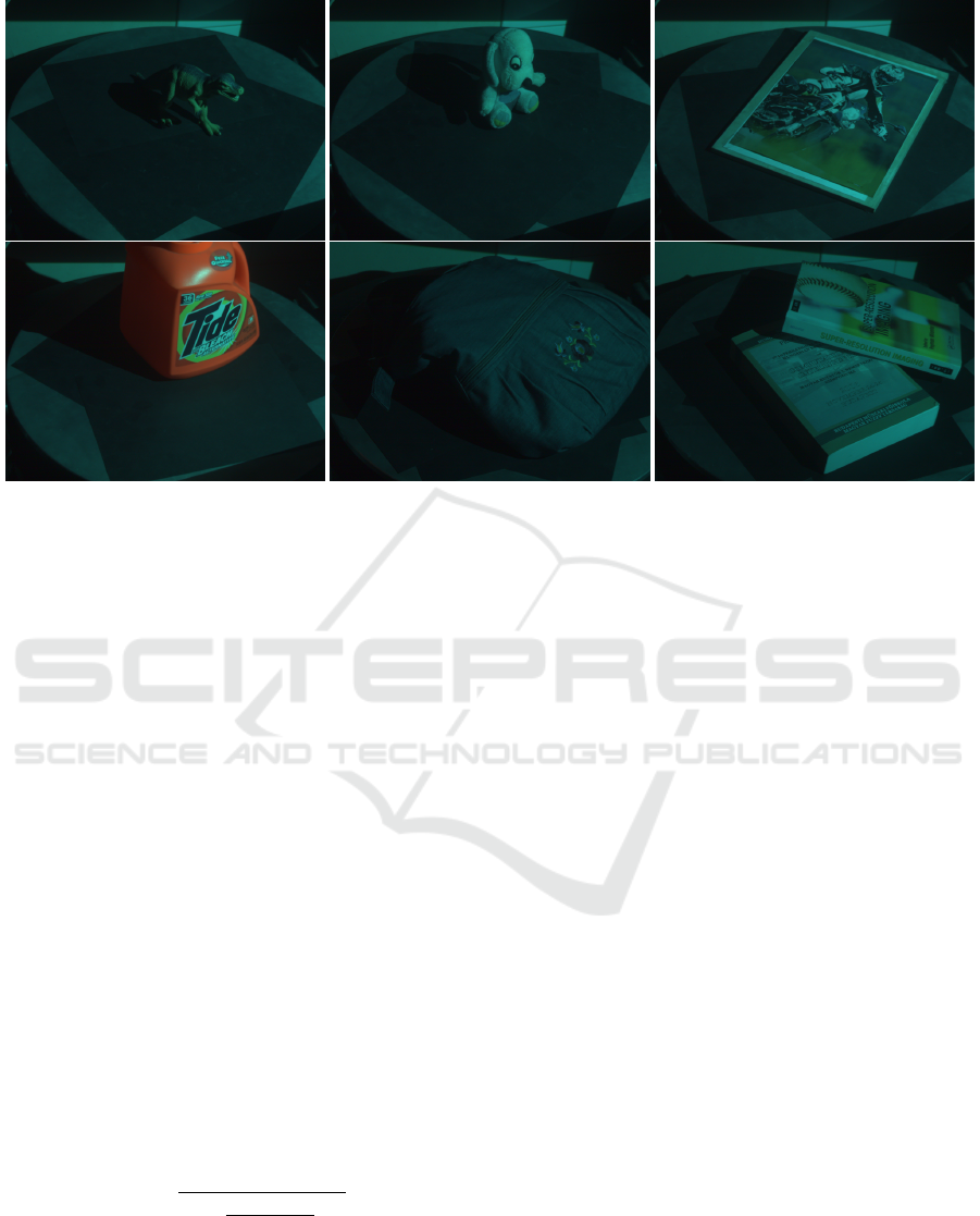
Figure 2: Objects used for testing. Upper row: Dino, PlushDog and Poster. Bottom row: Tide, Bag and Books.
of the eigenvalues define the length of the axes, and
the eigenvectors define the orientations of the ellipse
and the corresponding local affine region. Then the
ellipse is transformed to a circle, and the method is re-
peated iteratively until the eigenvalues of the second-
moment matrix are equal. This results the Harris-
Affine (HARAFF) and Hessian-Affine (HESAFF) de-
tectors (Mikolajczyk and Schmid, 2002). One of its
main benefits is that they are invariant to large view-
point changes.
Maximally Stable Extremal Regions (MSER) is
proposed by Matas et al. (Matas et al., 2002). This
method uses a watershed segmentation algorithm and
selects regions which are stable over varying lighting
conditions and image transformations. The regions
can have any formation, however an ellipse can be
easily fit by computing the eigenvectors of the second
moment matrices.
The Intensity Extrema-based Region (IBR) detec-
tor (Tuytelaars and Gool, 2000) selects the local ex-
temal points of the image. The affine regions around
these points are selected by casting rays in every di-
rection from this points, and selecting the points lying
on these rays where the following function reaches the
extremum:
f (t) =
|I(t) − I
0
|
max(
R
t
0
|I(t)−I
0
|dt
t
,d)
,
where I
0
, t, I(t) and d are the local extremum, the pa-
rameter of the given ray, the intensity on the ray at the
position and a small number to prevent the division
by 0, respectively. Finally, an ellipse is fitted onto this
region described by the points on the rays.
The Edge-based Region (EBR) detector (Tuyte-
laars and Van Gool, 2004) finds corner points P using
the Harris corner detector (Harris and Stephens, 1988)
and edges by the Canny edge detector (Canny, 1986).
Then two points are selected on the edges meeting
at P. This three points define a parallelogram whose
properties are studied. The points are selected as fol-
lows: the parallelogram that results the extemum of
the selected photometric function(s) of the texture is
determined first, then an ellipse is fitted to this paral-
lelogram.
The Speeded-Up Robust Features (SURF) (Bay
et al., 2008) uses box filters to approximate the Lapla-
cian of the Gaussian instead of computing the Differ-
ence of Gaussian like SIFT (Lowe, 2004) does. Then
it considers the determinant of the Hessian matrix to
select the location and scale.
Remark that the Harris-Hessian-Laplace
(HARHES) detector finds a large number of
points because it merges the feature points from
HARLAP and HESLAP.
4 EVALUATION METHOD
The feature detectors described in the previous sec-
tion detect features that can be easily tracked. Some
of the methods have their own descriptors, which are
used together with a matcher to match the correspond-
ing features detected on two successive images. How-
ever, some of them does not have this kind of descrip-
tors, so a different matching approach were used.
VISAPP 2017 - International Conference on Computer Vision Theory and Applications
518

4.1 Matching
A detected affine region around a feature point is de-
scribed by an ellipse calculated from the second mo-
ment matrix M:
M =
∑
x,y
w(x,y)∗

I
2
x
I
x
I
y
I
x
I
y
I
2
y

= R
−1

λ
1
0
0 λ
2

R, (1)
where w(x,y) and R are the Gussian filter and the rota-
tion matrix, respectively. The ellipse itself is defined
as follows:

u v

M

u
v

= 1
Since matrix M is always symmetric, 3 parameters are
given by the detectors: m
11
= I
2
x
, m
12
= m
21
= I
x
I
y
and m
22
= I
2
y
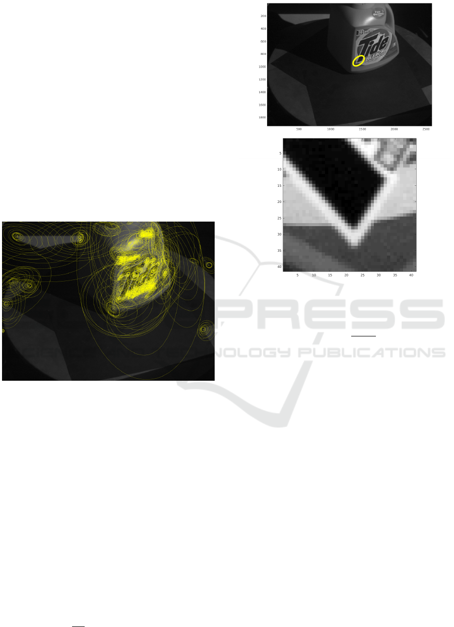
. Figure 3 shows some of the affine re-
gions, visualized by yellow ellipses on the first im-
age of the Flacon image set. The matching algorithm
Figure 3: The yellow ellipses show the affine regions on the
Flacon image.
uses these ellipses to match the feature points between
images. For each feature point, the second moment
matrix is calculated using the ellipse parameters, then
the square root of the inverse second moment matrix
transforms these ellipses into unit circles. This trans-
formation is scaled up to circles with the radius of 20
pixels, and rotated to align the minor axis of the el-
lipse to the x axis. Bilinear interpolation is used to
calculate the pixels inside the circles. The result of
this transformation can be seen in Figure 4. After the
normalization is done for every feature on two succes-
sive images, the matching can be started. The rotated
and normalized affine regions are taken into consid-
eration and a score is given which represent the simi-
larity between the regions. We chose the Normalized
Cross-Correlation (NCC) which is invariant for inten-
sity changes and can be calculated as follows:
NCC( f ,g) =
1
N1
∑
[ f (x,y) −
¯
f ] · [g(x,y) − ¯g],
Figure 4: The yellow ellipse (above) shows the detected
affine region. Below, the rotated and normalized affine re-
gion of the same ellipse can be seen.
were
N
1
=
p
S
f
· S
g
,
S
f
=
∑
[ f (x,y) −
¯
f ]
2
,
S
g
=
∑
[g(x,y) − ¯g]
2
.
The intervals of the sums are not marked since f and
g indicates the two normalized image patches whose
correlation needs to be calculated, and in our case
these two patches has a resolution of 41× 41 pixels.
¯
f
and ¯g denote the average pixel intensities of the patch
f and g, respectively. The NCC results a value in the
interval [−1,1]. 1 is given if the two patches are cor-
related, −1 if they are not.
For every affine region on the first image, a pair is
selected from the second image, which has the maxi-
mal NCC value. Then this matching needs to be done
backwards to eliminate the false matches. So an affine
region pair is selected only if the best pair for the first
patch A is B on the second image and the best pair
for B is A on the first image. Otherwise the pair is
dropped and marked as false match.
4.2 Error Metric
In this comparison we can only measure the error that
the detectors perpetrate, so detectors which find a lot
Quantitative Comparison of Affine Invariant Feature Matching
519

of feature points yield more error than detectors with
less feature points. Moreover false matches increase
this error further. Thus a new comparison idea is in-
troduced which can handle the problems above.
The error metric proposed by us (Pusztai and Ha-
jder, 2016a) is based on the weighted distances be-
tween the feature point found by the detector and the
GT feature points calculated from the previous loca-
tions the same feature. This means that only one GT
point appears on the second image, and the error of
the feature point on the second image is simply the
distance between the feature and the corresponding
GT point. On the third image, one more GT point
appears, calculated from the appearance of the same
feature on the first and on the second image. The error
of the feature on the third image is the weighted dis-
tance between the feature and the two GT points. The
procedure is repeated until the feature disappears.
The minimum (min)/maximum (max)/sum
(sum)/average (avg)/median (med) statistical values
are then calculated from the errors of the features per
image. Our aim is to characterize each detector using
only one value which is the average of these values.
See our paper (Pusztai and Hajder, 2016a) for more
details on the error metric.
5 THE COMPARISON
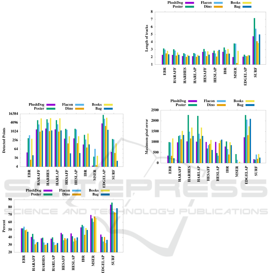
The first issue we discuss is the detected number of
features on the test objects. Features which were
detected on the other parts of the images were ex-
cluded, because only the objects were rotating. Fig-
ure 6 shows the number of features and that of inliers.
It is obvious that the EDGELAP found more number
of features than the others, and has more number of
inliers than the other detectors. However, it can be
seen in Figure 6 that SURF has the largest inlier ra-
tio – the percentage of the inliers – and EDGELAP
is almost the lowest. MSER has placed on the sec-
ond on this figure, however if we look at the row of
MSER in Figure 6, one can observe that MSER found
only a few feature points on the images, moreover
MSER found no feature point on the images of the
Bag. Few number of feature points is a disadvantage,
because they cannot capture the whole motion of the
object, but too high number of feature points can be
also a negative property, because they can result bad
matches (outliers).
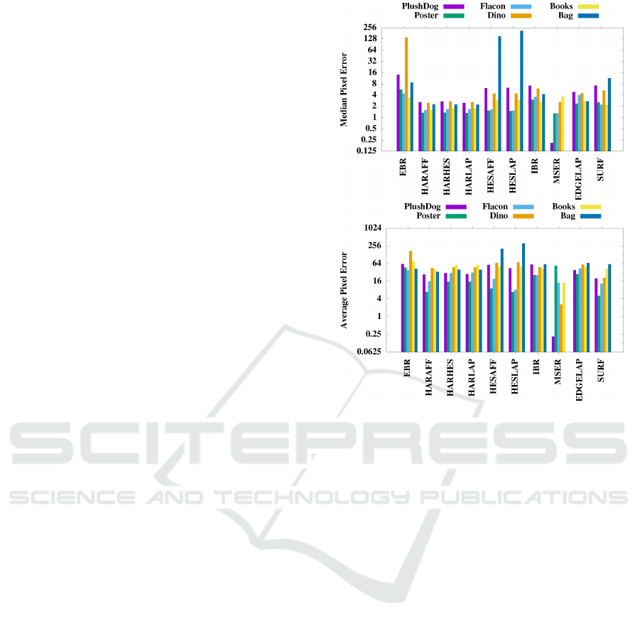
Figure 5 shows the median and average pixel er-
rors on a log scale. It is conspicuous that MSER
reaches below 1 pixel error on the PlushDog test ob-
ject, however as we mentioned above, that MSER
found only a couple of feature points on the Plush-
Figure 5: The median(above) and average(below) errors for
all methods of all test cases.
Dog sequence (below 5 in average), but these feature
points appears to be really reliable and easy to follow.
The average error of these trackers is around 16 pix-
els, while the median is around 2 pixels. Most of the
errors of the feature points are lower than 2 pixels,
however if the matching fails at some point, the error
grows largely. One can also observe the differences
between the test object. Obviously the small and low-
texture objects, like the Dino and the Bag are hard to
follow and indicate more errors than the others, while
Books, Flacon and Poster result the lowest errors.
It is hard to choose the best, but one can say that,
HARAFF, HARHES and HARLAP has low average
and median pixel errors, they found 1000 to 5000 fea-
tures on the images with a 30% inlier ratio. It is not
surprising that feature detectors based on the second-
moment matrix are more reliable than detector based
on the Hessian matrix, because the second moment
matrix is based on first derivatives, while the Hessian
matrix is based on second derivatives.
It must be noted that if we take a look on the
length of the feature tracks, eg. the average number
of successive images a feature point is being followed,
SURF performs highly above the other. In Figure 7,
it can be seen that SURF can follow a feature point
trough 5 or 6 images, while the other detectors do it
at most trough three images. The degree of rotation
VISAPP 2017 - International Conference on Computer Vision Theory and Applications
520

between the images was 3
◦
, which means that feature
points will not disappear so rapidly, thus the detectors
should have follow them longer.
The IBR and EBR detectors found less feature
points than the methods based on the Harris matrix,
but their inlier ratio was about 50%. However they re-
sulted more errors both for average and median. This
was true especially for EBR. The paper (Tuytelaars
and Van Gool, 2004) mentions that the problem with
EBR is that edges can change between image pairs,
they can disappear or their orientations can differ, but
IBR can complement this behavior. In our test cases
it turns out that IBR results slightly less errors than
EBR.
Figure 6: The detected number of features (above) and the
inlier ratio (below) in the test cases.
6 CONCLUSION
In this paper, we extended our work (Pusztai and Ha-
jder, 2016a) by comparing affine feature detectors.
Ground truth data were considered for six real-world
objects and a quantitative comparison was carried out
for the most popular affine feature detectors. The
matching of features generated on successive images
was done by normalizing the affine regions and using
Normalized Cross-Correlation for error calculation.
Our evaluation results show that HARAFF, HARHES
Figure 7: The average length of feature tracks.
Figure 8: The average of the maximum feature errors.
and HARLAP obtain the lowest tracking error, they
are the most accurate feature matchers, however, if
the length of the successfully tracked feature tracks
are considered, SURF is suggested. Only the errors
obtained by the location of feature points are consid-
ered in this paper, the accuracy of the detected affine
regions are not compared. In the future, we plan to ex-
tend this paper by comparing these affine regions us-
ing novel GT data considering affine transformations
between images.
REFERENCES
Agrawal, M. and Konolige, K. (2008). Censure: Center
surround extremas for realtime feature detection and
matching. In ECCV.
Alcantarilla, P. F., Bartoli, A., and Davison, A. J. (2012).
Kaze features. In Proceedings of the 12th European
Conference on Computer Vision, pages 214–227.
Baker, S., Scharstein, D., Lewis, J., Roth, S., Black, M.,
and Szeliski, R. (2011). A database and evaluation
methodology for optical flow. International Journal
of Computer Vision, 92(1):1–31.
Bay, H., Ess, A., Tuytelaars, T., and Gool, L. J. V. (2008).
Speeded-up robust features (SURF). Computer Vision
and Image Understanding, 110(3):346–359.
Quantitative Comparison of Affine Invariant Feature Matching
521

Beaudet, P. (1978). Rotational invariant image operators.
Proceedings of the 4th International Conference on
Pattern Recognition, pages 579–583.
Canny, J. (1986). A computational approach to edge de-
tection. IEEE Transactions on Pattern Analysis and
Machine Intelligence.
F
¨
orstner, W. and G
¨
ulch, E. (1987). A Fast Operator for De-
tection and Precise Location of Distinct Points, Cor-
ners and Centres of Circular Features.
Grauman, K. and Leibe, B. (2011). Visual Object Recogni-
tion. Synthesis Lectures on Artificial Intelligence and
Machine Learning. Morgan & Claypool Publishers.
Harris, C. and Stephens, M. (1988). A combined corner
and edge detector. In In Proc. of Fourth Alvey Vision
Conference, pages 147–151.
Leutenegger, S., Chli, M., and Siegwart, R. Y. (2011).
Brisk: Binary robust invariant scalable keypoints. In
Proceedings of the 2011 International Conference on
Computer Vision, ICCV ’11, pages 2548–2555.
Lowe, D. G. (1999). Object recognition from local scale-
invariant features. In Proceedings of the International
Conference on Computer Vision, ICCV ’99, pages
1150–1157.
Lowe, D. G. (2004). Distinctive image features from scale-
invariant keypoints. International Journal of Com-
puter Vision, 60(2):91–110.
Mair, E., Hager, G. D., Burschka, D., Suppa, M., and
Hirzinger, G. (2010). Adaptive and generic corner de-
tection based on the accelerated segment test. In Pro-
ceedings of the 11th European Conference on Com-
puter Vision: Part II, pages 183–196.
Matas, J., Chum, O., Urban, M., and Pajdla, T. (2002). Ro-
bust wide baseline stereo from maximally stable ex-
tremal regions. In Proc. BMVC, pages 36.1–36.10.
doi:10.5244/C.16.36.
Mikolajczyk, K. and Schmid, C. (2002). An affine invariant
interest point detector. In Proceedings of the 7th Eu-
ropean Conference on Computer Vision-Part I, ECCV
’02, pages 128–142, London, UK, UK. Springer-
Verlag.
Mikolajczyk, K., Tuytelaars, T., Schmid, C., Zisserman, A.,
Matas, J., Schaffalitzky, F., Kadir, T., and Gool, L. V.
(2005). A comparison of affine region detectors. In-
ternational Journal of Computer Vision, 65(1):43–72.
Morel, J.-M. and Yu, G. (2009). Asift: A new framework for
fully affine invariant image comparison. SIAM Jour-
nal on Imaging Sciences, 2(2):438–469.
Pablo Alcantarilla (Georgia Institute of Technology), Jesus
Nuevo (TrueVision Solutions AU), A. B. (2013). Fast
explicit diffusion for accelerated features in nonlinear
scale spaces. In Proceedings of the British Machine
Vision Conference. BMVA Press.
Pal, C. J., Weinman, J. J., Tran, L. C., and Scharstein, D.
(2012). On learning conditional random fields for
stereo - exploring model structures and approximate
inference. International Journal of Computer Vision,
99(3):319–337.
Pusztai, Z. and Hajder, L. (2016a). Quantitative Com-
parison of Feature Matchers Implemented in
OpenCV3. In Computer Vision Winter Work-
shop. vailable online at http://vision.fe.uni-
lj.si/cvww2016/proceedings/papers/04.pdf.
Pusztai, Z. and Hajder, L. (2016b). A turntable-based ap-
proach for ground truth tracking data generation. VIS-
APP, pages 498–509.
Rosten, E. and Drummond, T. (2005). Fusing points and
lines for high performance tracking. In In Internation
Conference on Computer Vision, pages 1508–1515.
Rublee, E., Rabaud, V., Konolige, K., and Bradski, G.
(2011). Orb: An efficient alternative to sift or surf.
In International Conference on Computer Vision.
Scharstein, D., Hirschm
¨
uller, H., Kitajima, Y., Krathwohl,
G., Nesic, N., Wang, X., and Westling, P. (2014).
High-resolution stereo datasets with subpixel-accurate
ground truth. In Pattern Recognition - 36th German
Conference, GCPR 2014, M
¨
unster, Germany, Septem-
ber 2-5, 2014, Proceedings, pages 31–42.
Scharstein, D. and Szeliski, R. (2002). A Taxonomy and
Evaluation of Dense Two-Frame Stereo Correspon-
dence Algorithms. International Journal of Computer
Vision, 47:7–42.
Scharstein, D. and Szeliski, R. (2003). High-accuracy
stereo depth maps using structured light. In CVPR
(1), pages 195–202.
Tomasi, C. and Shi, J. (1994). Good Features to Track. In
IEEE Conf. Computer Vision and Pattern Recognition,
pages 593–600.
Tuytelaars, T. and Gool, L. V. (2000). Wide baseline stereo
matching based on local, affinely invariant regions. In
In Proc. BMVC, pages 412–425.
Tuytelaars, T. and Van Gool, L. (2004). Matching widely
separated views based on affine invariant regions. Int.
J. Comput. Vision, 59(1):61–85.
Wu, J., Cui, Z., Sheng, V., Zhao, P., Su, D., and Gong, S.
(2013). A comparative study of sift and its variants.
Measurement Science Review, 13(3):122–131.
Zhang, Z. (2000). A flexible new technique for camera
calibration. IEEE Trans. Pattern Anal. Mach. Intell.,
22(11):1330–1334.
VISAPP 2017 - International Conference on Computer Vision Theory and Applications
522