A Dataset and a Comparison of Out-of-Order Event Compensation

Algorithms

Wolfgang Weiss, V

ıctor Juan Exp

osito Jim

enez and Herwig Zeiner

DIGITAL – Institute for Information and Communication Technologies,

JOANNEUM RESEARCH Forschungsgesellschaft mbH, Graz, Austria

Keywords:

Distributed Systems, Out-of-Order Event Compensation, Event Processing.

Abstract:

Event processing is order and time sensitive and therefore assumes temporally correct ordered event streams,

even in distributed systems, to be able to create correct results. In this work we discuss implementations of

four different out-of-order event compensation algorithms that use different kinds of dynamic time-out buffer-

ing techniques, and we compare those to a static buffering method. This is an approach which is generally

applicable and easy to integrate for existing distributed systems such as for Internet of Things applications.

For the evaluation, speciﬁc datasets were recorded, which are introduced in this paper, and which are freely

available under a Creative Commons license. Results show, that even with a restrictive buffer setting, most of

the out-of-order events can be compensated. Dynamic time-out buffering is still a trade-off between reaction

time and out-of-order event compensation, but it is useful in various applications.

1 INTRODUCTION

Distributed systems consist of spatially separated

nodes or processes which communicate with each

other via messages over computer networks. The

same applies for Internet of Things applications,

which can be considered as an inherently distributed

system generating and processing data. In event-

driven architectures this data is referred to as events

rather than as simple data points. Opher Etzion and

Peter Niblett (Etzion and Niblett, 2011) deﬁne an

event as something that has happened with an ac-

tual occurrence within a particular system or domain.

The continuous generation of events is called an event

stream or a time series of events.

In nowadays applications, such as for most Inter-

net of Things applications, it is no longer sufﬁcient to

store data and retroactively process it, but rather pro-

cess data online and make decisions near real-time.

To be able to do so, a processing agent, such as an

event processing engine, collects the event streams

from different sources and processes them. This

raises a couple of issues, mainly introduced by var-

ious delays, e.g. when detecting events, transferring

events to its destinations, or processing events. Sup-

pose you are searching for a pattern of event A being

followed by event B, with each event coming from a

different source in a distributed system. This requires

that all delays are either zero or of constant length,

otherwise it is likely that out-of-order events occur.

These are events which arrive too late, e.g. in our

example event A occurred before event B but arrived

after event B in the event processing engine. Event

processing is order and time sensitive and therefore

assumes temporally correct ordered event streams to

be able to create correct results. Consequences are:

• Missed events: no event detected when an event

should have been detected.

• False positives: detected an event when no event

should have been detected.

• Wrong calculations: a wrong value is calculated

when using a time window.

Possible solutions to handle out-of-order events:

• Time-out buffering: events are delayed in a buffer

until they reach a preset time-out. Events arriving

after the time-out cannot be compensated. This

generates a further delay to the whole processing

chain, and it is still not guaranteed that all out-of-

order event occurrences will be compensated.

• Retrospective compensation (undo / redo): if an

out-of-order event is detected, then all affected

and previously derived events must be retracted

(undo), and the processing must be started again at

the occurrence of the detected out-of-order event

Weiss, W., Jiménez, V. and Zeiner, H.

A Dataset and a Comparison of Out-of-Order Event Compensation Algorithms.

DOI: 10.5220/0006235400360046

In Proceedings of the 2nd International Conference on Internet of Things, Big Data and Security (IoTBDS 2017), pages 36-46

ISBN: 978-989-758-245-5

(redo). As there are no transaction mechanisms

available in current event processing systems, the

logic for this must be implemented individually.

• Identifying gaps with sequence numbers: every

event gets a sequence number while it is gener-

ated in the event producer. This allows the event

processing agent to recognize if there is a gap in

the event stream. This method works only for one

event producer and not in a distributed system.

To enable the detection of out-of-order events in a

distributed system, it is necessary to introduce clocks

and assign timestamps to events. Handling time and

therefore clocks in a distributed system introduces

a couple of problems. It is necessary to guarantee

that all event producers use the same time. Solutions

therefore could be to synchronize the clocks (e.g.

by using the Network Time Protocol (NTP) (Mills,

2010)) of the event producers or, that all event pro-

ducers use the same clock (e.g. using the GPS time

or a time server). NTP synchronizes the clocks in a

predeﬁned interval, but clocks may drift on their own,

and the synchronization process has some inaccura-

cies too. The second approach is not always avail-

able, has some latency and might create varying time

stamps. In general, it depends on the purpose and the

temporal granularity at which events are produced, to

be able to decide if one of the above mentioned meth-

ods is feasible. (cf. (Etzion and Niblett, 2011, pp.

291 - 295), (Della Valle et al., 2013), (Neville-Neil,

2015)).

To illustrate the importance of temporally correct

event streams, we have the following scenario from

the domain of connected cars in mind. Suppose there

is a multi-lane road with two cars each driving side

by side in the same direction. The cars scan the road

in front of them and report important observations to

the cars behind them over a wireless ad hoc network.

The right lane car at the head of the convoy detects

a person on the road 200 meters in front of it. At a

speed of 80 km/h this will not require any immediate

action, but this occurrence should be reported to the

other cars by alerting them: Event 1 (car 1, right lane,

person on the lane, 200m). The leading car on the left

lane receives this event and reports that its lane is free

for the next 300 meters: Event 2 (car 2, left lane, lane

is clear, 300m). The person moves on, causing the

cars to report following events: Event 3 (car 1, right

lane, person on the lane, 175m), and another report

by the car on the left lane: Event 4 (car 2, left lane,

lane is clear, 300m). The person reaches the left lane:

Event 5 (car 2, left lane, person on the lane, 150m).

Now, the right lane is free: Event 6 (car 1, right lane,

lane is clear, 300m).

The vehicles following car 1 and car 2 must ensure

to process those events timely and in the correct tem-

poral order to react fast and adequately. If the events

are in correct temporal order, they can infer following

information: The right lane is clear for the next 300

meters, while on the left lane there is a person in a

distance of 150 meters, and there is a person moving

from right to left. This example illustrates a use case

where the order of events is of signiﬁcant importance

and where a minimum delay is required for further ac-

tions. This use case also has multiple event producers

which work independently of each other.

In this work we want to ﬁnd answers to follow-

ing questions: Is there a dynamic buffering method

which is preferred over a static buffer? Is a dynamic

buffering method applicable in an Internet of Things

application? The expectations for an ideal buffer are

high. The buffer should be as small as possible and as

large as necessary so that all incoming events can be

fully re-ordered. The buffer should adapt itself to en-

vironmental changes, such as varying network delays

or other inﬂuences. Subsequently, we discuss the im-

plementation of four different out-of-order compensa-

tion algorithms, which use different kinds of dynamic

time-out buffering techniques and compare those to

an algorithm using a static buffering method. This is

a generally applicable and easy to integrate approach

for existing distributed applications. For the evalu-

ation, speciﬁc datasets were recorded which are in-

troduced in this paper, and which are freely available

under a Creative Commons license.

The next section gives an overview of existing and

related work in the ﬁeld of out-of-order event pro-

cessing and compensation. The content of the dataset

for evaluating out-of-order event compensation algo-

rithms is discussed in Section 3. Section 4 describes

the out-of-order compensation algorithms. The re-

sults of the evaluation are discussed in detail in Sec-

tion 5 and, ﬁnally, Section 6 concludes this work.

2 RELATED WORK

The authors in (Mutschler and Philippsen, 2013a)

present a system for reliable, low-latency, and dis-

tributed out-of-order event processing for use cases

with high data rates of events. They use a K-slack

buffer approach where the buffer length (K) is contin-

uously recalculated and adjusted. Events are delayed

for K time units at most, and within this timeframe

events can be reordered. The result is a correctly or-

dered event stream with minimal delay. This system

does not use a local or global clock but instead de-

rives the current time by incoming events. This ap-

proach has given us a basis to design some of our al-

A Dataset and a Comparison of Out-of-Order Event Compensation Algorithms

gorithms, but with improvements on the buffer size

calculation. In (Mutschler and Philippsen, 2013b),

the same authors extend their work on Low-Latency

constraint systems, and the look at the question of

how out-of-order events can be compensated by us-

ing the different delays between hosts in distributed

systems, thereby choosing the best route compensat-

ing for the delays to guarantee the correct event order.

The work of (Li et al., 2007) introduces a new

method to handle out-of-order events. It explains how

the proposed algorithm uses Active Instance Stacks

(AIS) (Wu et al., 2006) in cases where new out-of-

order events have been received by the system. The

AIS is a data structure which not only stores the cur-

rent instance status, but also the previous one. The al-

gorithm stores prevent AISs until the amount of cur-

rent event time unit, window length and K length is

less than the highest time unit received. If this hap-

pens, the system will be able to safely purge this

event. In our work, we don’t just store the pre-

vious event but also a limited time window which

improves the buffer size precision. In (Chen and

omer, 2013), the authors explain an algorithm to use

with out-of-order Parallel Discrete Event Simulation

(PDES). This algorithm uses predictive tables to avoid

conﬂicts between segments and predict next steps in

simulations. These predictions help the out-of-order

PDES to minimize the false conﬂicts. Finally, they

compare the optimized simulation in different situa-

tions to afﬁrm that the simulations increase the speed

over 1.8x.

Another domain in which the out-of-order com-

pensation is a sensitive issue is in audio and video ap-

plications. Addressing that, the paper (Arthur et al.,

2004) explains how the Transmission Control Proto-

col (TCP) degrades its performance in situations of

high packet reordering. The TCP uses sequence IDs

to re-order data packets on layer 4 (Transport Layer)

of the OSI model. This works reliably for network

data packets per network connection, meaning the re-

ordering is done for one source. In comparison to our

work, we do the re-ordering on layer 7 (Application

Layer) for several sources in a distributed system such

as an Internet of Things application.

3 DATASETS

3.1 Introduction

In this section we introduce the datasets we have

recorded with the purpose of evaluating out-of-order

event compensation algorithms. These are synthet-

ically generated datasets using standard commercial

devices, networks, and protocols commonly used in

Internet of Things applications aiming to resemble

real world use cases. Several sessions were carried

out to cover the inﬂuence of different parameters of

payload and network types. All datasets were made

open source and they are available to download on

our GitHub site

The datasets were designed to resemble the be-

havior and architecture of an Internet of Things use

case, where many nodes are connected over a net-

work. Each node continuously sends text-based mes-

sages to a common destination in a predeﬁned interval

over HTTP. The event producers are various kinds of

Android smartphones, running a customized applica-

tion which is optimized for efﬁcient event generation.

Two Windows PCs were also used as event producers

for the WLAN datasets running the same code base.

Details of the hardware and software conﬁguration

of the used devices are provided in the tables 1 and

2. The sessions were recorded using either the inter-

nal wireless network after the IEEE 802.11 standard

(WLAN), or the public cell phone network (UMTS)

of different providers.

Whenever a temporally correct ordered time-

series event stream in a distributed system is required,

all nodes must be synchronized. A common approach

is to synchronize the clocks of all nodes and assign

timestamps to the events. The Network Time Protocol

(NTP) (Mills, 2010) was evaluated for this purpose.

A NTP client is already included in Android, but we

have no inﬂuence on the synchronization without root

permissions, which makes this variant useless for our

approach. A simpler variant is the Simple Network

Time Protocol (SNTP), but evaluations revealed that

this variant is too imprecise for our use case. An-

other interesting method could have been the usage of

vector clocks (Mattern, 1989). This algorithm does

not need any centralized time server, since it uses lo-

cal synchronized time to know when an event is an

out-of-order event. Unfortunately, it adds too much

complexity, as many sensors are involved in the sys-

tem, due to the exponential growth of messages when

an event is corrected. For this reason, we have im-

plemented our own solution where clients request the

server time via HTTP and then calculate the time dif-

ference to their internal clock. In more detail, to get

a properly synchronized clock, we queried the server

ten times and then calculated the median offset to the

server time. This synchronization mechanism uses a

similar methodology to the one used by the Precision

Time Protocol (PTP) (IEE, 2008). The synchroniza-

tion process is executed before the start of each ses-

sion.

https://github.com/JR-DIGITAL/ooo-dataset

IoTBDS 2017 - 2nd International Conference on Internet of Things, Big Data and Security

Figure 1 shows the whole process starting from

the client’s detection of an event until it receives the

response from the server. The following timestamps

are involved:

• Detection time (dt): the time when the client de-

tects an event.

• Client send time (cst): the time when the message

leaves the client.

• Server receive time (srect): the time when the

server receives the event.

• Server response time (srest): the time when the

internal processing of the server is ﬁnished and

sends its response to the client.

• Client receive time (crt): the time when the client

receives the response from the server.

The following relevant durations can be derived

from these timestamps:

• Message preparation time: the duration between

the client’s detection of an event and its sending

of the message to the server (cst − dt).

• Server processing time: the duration the server

needs to process the message (srest − srect).

• Transmission time: (tt) the duration between

the event is detected until it reaches the server

(srect − dt).

• Network round-trip time: (RT T ) the duration

where the message is on the network (srect −

cst) + (crt − srest).

• Full processing time: this includes the preparation

time of the message, network round-trip time and

server processing time (crt − dt).

Figure 1: Chronological sequence from detecting an event

until the response is received by the client.

While recording a dataset, each client created its

own log ﬁle on the local device which contains all lo-

cally generated timestamps and settings. The server

logged all incoming message with additional times-

tamps into the server-side log ﬁle. After the recording

was ﬁnished, all log ﬁles were collected and merged

into one log ﬁle. This merged log ﬁle represents one

dataset and contains all necessary information to fully

reproduce all out-of-order events that have occurred.

A dataset contains following attributes:

• Device ID: a unique ID to identify each client.

• Sequence ID: (sid) an ascending serial number

which is unique for each message per client.

• Detection Time: (dt)

• Client send time: (cst)

• Client receive time: (crt)

• Server receive time: (srect)

• Server response time: (srest)

• Server processing time

• Message size: the size of the whole message in-

cluding payload and headers.

• Session Name: a name to identify the session

• Network type: UMTS or WiFi

• Time of the last time synchronization: time when

the client executed the clock synchronization.

• Synchronization time offset (ms): clock synchro-

nization offset between server’s clock and client’s

clock.

• Additional payload: the additional added pay-

load.

The datasets allow us to use two different ways

to identify an event as an out-of-order event. The

ﬁrst is by using the sequence ID, which allows to

identify out-of-order events per each client. Assume

we have an event stream of e

, e

, ..., e

which is or-

dered ascending by the sequence ID e

.sid < e

i+1

.sid,

(1 ≤ i < n). In this case we can identify an out-of-

order event e

if there is an event e

with 1 ≤ i < j ≤ n

and e

.sid > e

.sid. Another approach, which is more

relevant in a distributed system, is to use the detec-

tion time dt. Therefore we assume an event stream

, e

, ..., e

, (1 ≤ i < n) which is ordered ascending

by the detection time e

.dt ≤ e

i+1

.dt. An out-of-order

event e

can be identiﬁed if there is an event e

with

1 ≤ i < j ≤ n and e

.dt > e

.dt.

3.2 Analysis

An overview of all recorded datasets is given in ta-

ble 3 and 4. The datasets were recorded in nine ses-

sions, with each session lasting 600 seconds. The

datasets D-1 to D-5 have been done over the pub-

lic cell phone network (UMTS) of different providers

with 7–9 clients. In these datasets, the clients sent

A Dataset and a Comparison of Out-of-Order Event Compensation Algorithms

an event to the server in an interval of 500ms. In each

session we used a different predeﬁned net payload be-

tween 0 bytes and 10KiB. This results in a bandwidth

for each client between 0.5KiB/s and 21.3KiB/s, and

a bandwidth on the server between 4.1KiB/s and

150KiB/s. The out-of-order events detected by using

the detection time ranges between 16.13% and 34.2%

of total events for each dataset.

The records S-7 to S-10 used our local WLAN

during working hours. The interval time between

events was set to 200ms. This results in a band-

width for the clients between 7KiB/s and 53KiB/s,

and for the server between 69KiB/s and 534 KiB/s.

Detected out-of-order events range between 19.91%

and 28.57% of total events for each dataset.

The amount of out-of-orders events for the WLAN

records (S-8 to S-10) is always higher than for the

UMTS data records (D1 to D5), this might be be-

cause of the lower interval of 200ms for the WLAN

dataset. The median and mean of the full processing

time (crt −dt) for the UMTS datasets is always higher

than the median and mean for the WLAN dataset.

4 ALGORITHMS

Four different algorithms for out-of-order event com-

pensation have been implemented in Java. All of them

use the detection time (dt) to identify out-of-order

events, as this is a suitable solution for distributed sys-

tems. The dynamic buffer algorithms continuously

recalculate the buffer size based on the transmission

times of the incoming events. Incoming event events

are kept in the buffer until dt +bu f f ertime is reached

and are emitted after this period. If the buffer time

is too small to correctly re-order an event, then it is

marked as not compensated and will be emitted im-

mediately. The aim for a dynamic buffer is to adapt

its buffer size according to the current environmental

situation e.g. the varying network delays. This allows

to keep the buffer time as small as possible while re-

ordering all incoming events. Subsequently we dis-

cuss the buffer size calculation of each proposed al-

gorithm.

4.1 Static Buffer Algorithm (SBA)

This algorithm uses a static, predeﬁned buffer time.

The Static Buffer Algorithm is included for compari-

son purposes to be able to evaluate the differences to

other algorithms.

4.2 Buffer Estimation based on Single

Transmission Time (BETT)

A dynamic value of the buffer time is nec-

essary to achieve a better performance even

when there are several changes on the network.

Therefore, this algorithm uses the transmis-

sion time (tt) of the latest event to adapt the

buffer size. If tt + o f f set is smaller than the

currentBu f f erTime, then the buffer time will be in-

creased: newBu f f erTime = (currentBu f f erTime ∗

increaseFactor) + o f f set. If tt + o f f set is big-

ger than the currentBu f f erTime + threshold,

then the buffer size will be decreased as fol-

lows: newBu f f erTime = currentBu f f erTime ∗

decreaseFactor. The increaseFactor and

decreaseFactor deﬁne to which extent the buffer size

will be changed.

4.3 Buffer Estimation based on

Transmission Time Average

(BETTA)

This algorithm also uses the transmission time (tt) to

calculate the buffer time, but in contrast to BETT it

keeps n transmission times in a temporal window of

predeﬁned length in milliseconds. This enables us

to get a baseline measure of the overall transmission

time. The arithmetic mean of this window is calcu-

lated and an offset is added:

bu f f erTime =

∑

i=1

+ o f f set (1)

4.4 Buffer Estimation based on

Transmission Time Weighted

Average (BETTWA)

This algorithm also uses a temporal window of prede-

ﬁned length in milliseconds containing n transmission

times to calculate a baseline of the overall network

delay. In this case we use a weighted mean with ex-

ponentially decreasing weights and add an offset.

bu f f erTime =

∑

i=1

(tt

∗ w

)

∑

i=1

+ o f f set (2)



n − i



(3)

IoTBDS 2017 - 2nd International Conference on Internet of Things, Big Data and Security

Table 1: Overview of the used client devices’ hardware, hardware conﬁguration and operating system.

Client ID Dataset Client ID Device Type OS Version Architecture Cores

1 dev 1 Huawei MediaPad 7 Zoll Android 4.0.3 SDK:15 armv7l 2

2 dev 2 Nexus S Android 4.1.2 SDK:16 armv7l 1

3 dev 3 PC Client Windows 7 amd64 4

4 dev 4 PC Client Windows 7 x86 2

5 dev 5 Motorola Android 4.1.2 SDK:16 i686 2

6 dev 6 Nexus 7 Tablet Android 4.4.4 SDK:19 armv7l 4

7 dev 7 Galaxy Nexus Android 4.3 SDK:18 armv7l 2

8 dev 8 Moto X Android 4.4.2 SDK:19 armv7l 2

9 dev 9 Samsung Galaxy Tab 2 Android 4.2.2 SDK:17 armv7l 2

10 dev 10 Samsung Galaxy Tab Android 4.0.4 SDK:15 armv7l 2

11 dev 11 Galaxy Nexus Android 4.4.4 SDK:19 armv7l 2

12 dev 12 LG-D802 Android 4.4.2 SDK:19 armv7l 4

13 dev 13 Nexus 5 Android 4.4.4 SDK:19 armv7l 4

14 dev 14 Samsung, GT-I9300 Android 4.3 SDK:18 armv7l 4

15 dev 15 Galaxy Nexus Android 4.4.4 SDK:19 armv7l 2

16 dev 16 Samsung, GT-I8190 Android 4.1.2 SDK:16 armv7l 2

Table 2: Overview of the used client devices’ brand, manufacturer and Java virtual machine.

Client ID Device Brand and Manufacturer Java Virtual Machine

1 Brand: Huawei, Model: HUAWEI MediaPad, Manufacturer: HUAWEI Dalvik version: 1.6.0

2 Brand: google, Model: Nexus S, Manufacturer: samsung Dalvik version: 1.6.0

3 Dell Laptop, Core I7 Java HotSpot(TM) 64-Bit Server VM version: 24.65-b04 (1.7.0 65)

4 Dell Laptop, Core 2 Duo Java HotSpot(TM) Client VM version: 24.65-b04 (1.7.0 65)

5 Brand: motorola, Model: XT890, Manufacturer: motorola Dalvik version: 1.6.0

6 Brand: google, Model: Nexus 7, Manufacturer: asus Dalvik version: 1.6.0

7 Brand: google, Model: Galaxy Nexus, Manufacturer: samsung Dalvik version: 1.6.0

8 Brand: motorola, Model: XT1052, Manufacturer: motorola Dalvik version: 1.6.0

9 Brand: samsung, Model: GT-P5110, Manufacturer: samsung Dalvik version: 1.6.0

10 Brand: samsung, Model: GT-P7500, Manufacturer: samsung Dalvik version: 1.6.0

11 Brand: google, Model: Galaxy Nexus, Manufacturer: samsung Dalvik version: 1.6.0

12 Brand: lge, Model: LG-D802, Manufacturer: LGE Dalvik version: 1.6.0

13 Brand: google, Model: Nexus 5, Manufacturer: LGE Dalvik version: 1.6.0

14 Brand: samsung, Model: GT-I9300, Manufacturer: samsung Dalvik version: 1.6.0

15 Brand: google, Model: Galaxy Nexus, Manufacturer: samsung Dalvik version: 1.6.0

16 Brand: samsung, Model: GT-I8190, Manufacturer: samsung Dalvik version: 1.6.0

Table 3: An overview of the recorded datasets describing the number of clients, used network, the payload, and the resulting

data rates.

ID Clients Network Interval (ms) Net Payload (Bytes) Gross Payload (Bytes) Events Server KiB/sec Clients KiB/sec

D-1 8 UMTS 500 0 265 9600 4.1 0.5

D-2 9 UMTS 500 512 1409 10800 24.8 2.8

D-3 8 UMTS 500 1024 1365 9600 21.3 2.7

D-4 7 UMTS 500 2048 2426 8400 33.2 4.7

D-5 7 UMTS 500 10240 10929 8400 149.4 21.3

S-7 10 WLAN 200 512 1409 30000 68.8 6.9

S-8 10 WLAN 200 1024 1365 30000 66.7 6.7

S-9 10 WLAN 200 2048 2426 29915 118.1 11.8

S-10 10 WLAN 200 10240 10929 29999 533.6 53.4

Table 4: The analysis of the recorded datasets describing the number of out-of-order events and a summary of the processing

times.

OoO Events Full Processing Time

ID Clients Network Number Percentage Min Q1 Median Mean Q3 Max Std Dev

D-1 8 UMTS 1548 16.13% 59 139 162 181.1 190 4738 103.9

D-2 9 UMTS 3693 34.19% 81 137 167 185.8 205 3680 115.6

D-3 8 UMTS 3283 34.20% 74 132 157 182.7 187 5616 183.8

D-4 7 UMTS 2321 27.63% 77 145 165 193.4 203 3300 116.5

D-5 7 UMTS 1591 18.94% 154 250 271 288.9 304 1911 83.7

S-7 10 WLAN 7795 25.98% 11 24 32 46.5 50 1522 49.9

S-8 10 WLAN 5974 19.91% 15 27 37 48.4 50 872 47.1

S-9 10 WLAN 7955 26.59% 15 29 39 52.6 54 3385 94.1

S-10 10 WLAN 8572 28.57% 46 75 92 103.7 114 1379 51.3

A Dataset and a Comparison of Out-of-Order Event Compensation Algorithms

4.5 Buffer Estimation based on

Transmission Time Difference

(BETTD)

In the best case, such a buffer has to compensate only

the variation of changes in the environment over time.

Assuming that all delays were of constant length,

there would be no out-of-order event. However, those

delays are not guaranteed, especially in wireless net-

works or in networks with a shared medium. There-

fore we calculate the maximum difference of trans-

mission times over a temporal window of predeﬁned

length and add an offset.

bu f f erTime = (max(tt) − min(tt)) +o f f set (4)

5 EVALUATION AND RESULTS

For the evaluation we used by way of example the

datasets D-5 and S-10, covering both network types

(UMTS and WLAN). The datasets are the ones with

the highest payload, and additionally, the dataset S-

10 has the highest absolute number of out-of-order

events. Moreover, they are evenly distributed over the

whole period of the recording in both datasets. We

determined suitable settings for the algorithms in var-

ious test runs and for the evaluation we used the same

settings on both datasets.

Following settings where used for the algorithms:

• Static Buffer Algorithm (SBA)

buffer time: 700ms

• Estimation based on single Transmission Time

(BETT)

initial buffer time: 500ms; threshold to decrease

the buffer 100ms; increase factor: 2; decrease fac-

tor: 0.99; offset time: 500ms

• Buffer Estimation based on Transmission Time

Average (BETTA) and Buffer Estimation based on

Transmission Time Weighted Average (BETTWA)

temporal window to calculate the average: 20

seconds; initial buffer time: 700ms; offset time:

700ms

• Buffer Estimation based on Transmission Time

Difference (BETTD)

temporal window to calculate the difference: 300

seconds; initial buffer time: 750ms; offset time:

350ms

The static buffer algorithm (SBA) is the baseline

for all other algorithms which do not dynamically

adapt their buffer size. This algorithm uses a ﬁxed

buffer size of 700ms. On dataset S-10 there are four

events out of 8572 out-of-order events which could

not be brought into correct order due to a too small

buffer size, and on dataset D-5 there were 17 events

out of 1591 out-of-order events which could not be

re-ordered (see also table 5).

The algorithm “buffer estimation based on sin-

gle transmission time (BETT)” uses the transmission

time of the latest event to calculate the optimal buffer

size. It performed well on dataset D-5 where it could

compensate all out-of-order events, but on dataset S-

10 it produced the worst results. The reason could be

that the variance of the transmission times in dataset

S-10 is much lower than for D-5 which also results

in a lower overall buffer size when applying this al-

gorithm on dataset S-10. The behavior of the buffer

over time is illustrated in ﬁgure 2 (a) for dataset D-5

and in ﬁgure 2 (b) for dataset S-10.

Calculating the buffer size for BETTA and

BETTWA works in a very similar manner, and the

results reﬂect this similarity. On dataset S-10 both

algorithms produced fairly good results but failed on

dataset D-5 because these algorithms do not adapt to

sudden changes of transmission times (see also ﬁgure

2 (c)). Additionally, the mean buffer size on S-10 is

the highest for this dataset. The transmission time’s

mean over a time window provides a good overall

measure of the current state of the network. Both al-

gorithms also suffer from a cold start problem, be-

cause at the beginning there is not enough data to cal-

culate a reliable mean. To provide useful results, these

algorithms need a fairly high offset.

To calculate the buffer size, the BETTD algorithm

uses the difference between the minimal and maxi-

mal transmission times over a time window, as, ide-

ally, all you have to compensate is the variance of the

transmission time. This algorithm needs a fairly big

temporal window of 300 seconds to work reliably and

hence suffers especially from the cold start problem.

As illustrated in ﬁgure 2 (d), it shows good adapta-

tion to transmission time changes. It has the ability to

adapt to sudden changes and therefore only needs - in

comparison to other algorithms - a fairly small offset

of 350ms.

We deliberately set the offset for all algorithms

as low as possible to make the limitations of each

algorithm clear. Hence, the key for re-ordering all

out-of-order events in all possible situations is to give

the algorithms enough offset, but this results in high

buffering times which might be unwanted. Accord-

ing to this aspect, the algorithm BETTD provided the

best overall results, as it needs a smaller offset value

than all other algorithms. For situations, where the re-

action time is more important than compensating all

out-of-order events, the BETTA algorithm might be

IoTBDS 2017 - 2nd International Conference on Internet of Things, Big Data and Security

Table 5: Evaluation results of the buffer algorithms: a summary of the buffer size (ms) and the number of compensated

out-of-order events.

Buffer Size (ms) Out-of-Order Events

Algorithm Dataset

Min Q1 Median Mean Q3 Max Std Dev. Compensated Not-Compensated

SBA D-5 700 700 700 700.0 700 700 0 1574 17 (1,07%)

BETT D-5 641 671 684 701.2 702 2048 111 1591 0 (0,00%)

BETTA D-5 700 788 791 793.9 794 1569 29 1582 9 (0,57%)

BETTWA D-5 700 785 790 793.1 794 1554 34 1583 8 (0,50%)

BETTD D-5 595 635 661 772.3 675 1982 350 1588 3 (0,19%)

SBA S-10 700 700 700 700.0 700 700 0 8568 4 (0,05%)

BETT S-10 583 608 611 628.5 620 1697 55 8565 7 (0,08%)

BETTA S-10 736 741 743 744.5 746 782 5 8571 1 (0,01%)

BETTWA S-10 735 741 742 744.1 746 794 7 8570 2 (0,02%)

BETTD S-10 390 863 892 943.8 951 1597 165 8570 2 (0,02%)

Figure 2: The buffer size (y-axis) of the used buffer algorithm (blue line) and the transmission time (y-axis) of events over

the session time (x-axis). Each dot represents the transmission time of an event and not compensated out-of-order events are

highlighted in red. (a) algorithm BETT on dataset D-5, (b) algorithm BETT on dataset S-10, (c) algorithm BETTA on dataset

D-5, (d) algorithm BETTD on dataset D-5.

the choice. This algorithm is stable over a long time,

neglects single outliers but still adapts to changes.

The evaluation showed that the datasets D-5 and

S-10 have different requirements to the adaptation of

the buffer time. They reveal different parameters (e.g.

the variance of transmission times) but no parame-

ter could be found which allows for the prediction of

sudden outliers. The criteria when a dynamic buffer

would be preferred over a static buffer are that the

overall delay is smaller, while re-ordering more out-

of-order events and that it is able to quickly adapt

its buffer size to even sudden environmental changes,

e.g. varying network delays. The higher the variation

of the network or other inﬂuences in the environment

is, the more necessary it is to use an algorithm which

dynamically adapts its buffer size, as a forecast of the

buffer size for a static buffer might be difﬁcult and not

always applicable. The use of buffering algorithms

is still a trade-off between reaction time and out-of-

order event compensation, but it is useful in various

applications.

A Dataset and a Comparison of Out-of-Order Event Compensation Algorithms

6 CONCLUSIONS

In this work we gave an introduction to the area of

processing event streams in distributed systems. As

event processing is order and time sensitive, we ex-

plained what problems arise when processing event

streams that include out-of-order events, and outlined

possible solutions.

We presented an evaluation of different time-out

buffering algorithms, which are general applicable,

easy to integrate in existing architectures and particu-

larly interesting for Internet of Things applications.

To be able to evaluate those algorithms we had to

record datasets ﬁrst, as we did not ﬁnd a freely avail-

able dataset with the desired features. The recording

of these datasets was carried out in several sessions on

WLAN and UMTS, with varying payload, and vari-

ous mobile devices. We publish these datasets under

a Creative Commons license to allow other develop-

ers to evaluate their approaches.

The implemented dynamic buffering algorithms

are able to adapt their buffer size to environmental

changes, such as varying network delays or other in-

ﬂuences. Those algorithms proved to produce better

results than a static buffer. The buffering algorithm

“buffer estimation based on transmission time differ-

ence (BETTD)” produced the best overall results as it

adapts to changes quickly and does not need much ad-

ditional offset. Another useful implementation might

be the variant “buffer estimation based on transmis-

sion time average (BETTA)”. This algorithm is sta-

ble over a long time, neglects single outliers but still

adapts to changes.

Time-out buffering is still a trade-off between re-

action time and out-of-order event compensation. Ul-

timately, it depends on the application how much de-

lay and how much out-of-order events are desired.

ACKNOWLEDGEMENTS

This research was funded by the Austrian Ministry

for Transport, Innovation and Technology (BMVIT)

within the framework of the sponsorship under

the project “Collaborative Robotics” (CollRob) and

“Multi-Dimensional Sensor Data Time Series Analy-

sis” (MUST). This research was also funded by the

Austrian research funding association (FFG) within

the research project “Monitoring and Analysis of

Heavy Machinery using non-intrusive Measurement

Techniques” (MAHMAMT).

REFERENCES

(2008). IEEE Standard for a Precision Clock Synchroniza-

tion Protocol for Networked Measurement and Con-

trol Systems. IEEE Std 1588-2008, pages 1–269.

Arthur, C. M., Girma, D., Harle, D., and Lehane, A. (2004).

The effects of packet reordering in a wireless multi-

media environment. In 1st Int. Symposium on Wireless

Communication Systems, pages 453–457.

Chen, W. and D

omer, R. (2013). Optimized out-of-order

parallel discrete event simulation using predictions. In

Design, Automation Test in Europe Conference Exhi-

bition (DATE), 2013, pages 3–8.

Della Valle, E., Schlobach, S., Kr

otzsch, M., Bozzon, A.,

Ceri, S., and Horrocks, I. (2013). Order matters! har-

nessing a world of orderings for reasoning over mas-

sive data. Semant. web, 4(2):219–231.

Etzion, O. and Niblett, P. (2011). Event Processing in

Action. Manning Publications Co., Greenwich, CT,

USA, 1st edition.

Li, M., Liu, M., Ding, L., Rundensteiner, E. A., and Mani,

M. (2007). Event stream processing with out-of-order

data arrival. In 27th Int. Conf. on Distributed Comput-

ing Systems Workshops, pages 67–67.

Mattern, F. (1989). Virtual time and global states of dis-

tributed systems. In Proc. Workshop on Parallel

and Distributed Algorithms, pages 215–226, North-

Holland / Elsevier.

Mills, D. L. (2010). Computer Network Time Synchroniza-

tion: The Network Time Protocol on Earth and in

Space, Second Edition. CRC Press, Inc., Boca Raton,

FL, USA, 2nd edition.

Mutschler, C. and Philippsen, M. (2013a). Distributed low-

latency out-of-order event processing for high data

rate sensor streams. In IEEE 27th Int. Symposium on

Parallel Distributed Processing, pages 1133–1144.

Mutschler, C. and Philippsen, M. (2013b). Runtime migra-

tion of stateful event detectors with low-latency order-

ing constraints. In IEEE Int. Conf. on Pervasive Com-

puting and Commun. Workshops, pages 609–614.

Neville-Neil, G. V. (2015). Time is an illusion lunchtime

doubly so. Commun. ACM, 59(1):50–55.

Wu, E., Diao, Y., and Rizvi, S. (2006). High-performance

complex event processing over streams. In Proceed-

ings of the 2006 ACM SIGMOD Int. Conf. on Man-

agement of Data, pages 407–418, New York. ACM.

APPENDIX

This section gives additional insight to the recorded

dataset. The following ﬁgures illustrate the transmis-

sion times for each event and highlight out-of-order

events. As described in section 3, the transmission

time is the duration between the event is detected un-

til it reaches the server (srect − dt).

IoTBDS 2017 - 2nd International Conference on Internet of Things, Big Data and Security

Figure 3: Each dot represents the transmission time of an

event of the dataset S-7, out-of-order events are highlighted

in red.

Figure 4: Each dot represents the transmission time of an

event of the dataset S-8, out-of-order events are highlighted

in red.

Figure 5: Each dot represents the transmission time of an

event of the dataset S-9, out-of-order events are highlighted

in red.

Figure 6: Each dot represents the transmission time of an

event of the dataset S-10, out-of-order events are high-

lighted in red.

Figure 7: Each dot represents the transmission time of an

event of the dataset D-1, out-of-order events are highlighted

in red.

Figure 8: Each dot represents the transmission time of an

event of the dataset D-2, out-of-order events are highlighted

in red.

A Dataset and a Comparison of Out-of-Order Event Compensation Algorithms

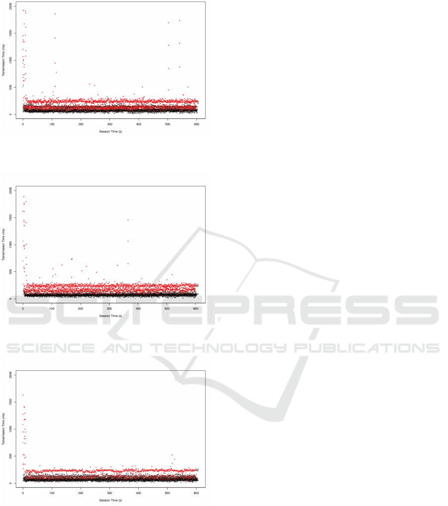
Figure 9: Each dot represents the transmission time of an

event of the dataset D-3, out-of-order events are highlighted

in red.

Figure 10: Each dot represents the transmission time of an

event of the dataset D-4, out-of-order events are highlighted

in red.

Figure 11: Each dot represents the transmission time of an

event of the dataset D-5, out-of-order events are highlighted

in red.

IoTBDS 2017 - 2nd International Conference on Internet of Things, Big Data and Security