
Part-driven Visual Perception of 3D Objects
Frithjof Gressmann, Timo L¨uddecke, Tatyana Ivanovska, Markus Schoeler and Florentin W¨org¨otter
Georg-August-University, G¨ottingen, Germany
tiva@phys.uni-goettingen.de
Keywords:
Object Recognition, Part Perception, Deep Learning, Neural Networks, 3D Objects.
Abstract:
During the last years, approaches based on convolutional neural networks (CNN) had substantial success in
visual object perception. CNNs turned out to be capable of extracting high-level features of objects, which
allow for fine-grained classification. However, some object classes exhibit tremendous variance with respect
to their instances appearance. We believe that considering object parts as an intermediate representation could
be helpful in these cases. In this work, a part-driven perception of everyday objects with a rotation estimation
is implemented using deep convolution neural networks. The used network is trained and tested on artifi-
cially generated RGB-D data. The approach has a potential to be used for part recognition of realistic sensor
recordings in present robot systems.
1 INTRODUCTION
The latest wave of artificial neural network methods
which was triggered by Krizhevsky et al. (2012) has
led to impressive progress on many computer vision
problems. However, CNNs can not compete with hu-
mans in terms of generalization. This can be exempli-
fied by looking at objects with a greatly varying ap-
pearance, e.g. power-drills. They come in vastly dif-
ferent forms and shapes (hand-held, on a stand, etc.)
and when comparing two drill objects as a whole,
many times there are only very few common visual
features across instances which could support suc-
cessful whole-object recognition with CNNs. The
fact that humans can refer to these objects as drills,
however, can be explained by looking at the object
parts: On a part level the two drill types share com-
parable features, e.g. the boring bit and the power-
switch and some others. This view suggests that a
visual scene understanding and the class recognition
in particular can be strongly guided by parts.
When it comes to handling and usage of objects,
an adequate understanding of the main functional ob-
ject parts seems to be indispensable. Particularly
knowledge about which objects parts are suitable for
grasping and manipulating forms are an important ba-
sis of the everyday life activities that robots are aim-
ing for. In this regard, the recent achievements of
convolutional neural networks suggest exploring the
potential of an object perception on a per-part basis.
To the best of our knowledge, so far, object recog-
nition with neural networks has been mainly focused
on whole object, approaches explicitly addressing
parts are rather uncommon, in particular in conjunc-
tion with 3D data, like depth images and normals
maps as input.
2 RELATED WORK
The idea of considering objects as composite struc-
tures involving many parts is not new to computer vi-
sion.
Perhaps most well known, Biederman (1987) sug-
gested the recognition by components (RBC) theory.
According to Biederman the human object recogni-
tion is carried out by separating objects into its main
components which he calls geons (Biederman, 1987).
An advantage of this approach is its economy since a
small number of basic parts can form a huge num-
ber of possible objects. Also, part recognition is
viewpoint-invariant to some degree since the prop-
erties of object parts do not change massively under
different viewing angles. However, RBC provides a
theoretical framework rather than an implementation,
whereas this work presents a concrete algorithm. It
shares with RBC the consideration of parts but our
parts are neither geons nor is the number of part
classes limited to 36. The segmentation of objects
into parts is addressed by Schoeler et al. (2015). They
propose a bottom-up algorithm to dissect objects into
parts based on local convexity which does not require
annotated training data.
In the 2D domain, the implicit shape model (Leibe
370
Gressmann F., LÃijddecke T., Ivanovska T., Schoeler M. and WÃ˝urgÃ˝utter F.
Part-driven Visual Perception of 3D Objects.
DOI: 10.5220/0006211203700377
In Proceedings of the 12th International Joint Conference on Computer Vision, Imaging and Computer Graphics Theory and Applications (VISIGRAPP 2017), pages 370-377
ISBN: 978-989-758-226-4
Copyright
c
2017 by SCITEPRESS – Science and Technology Publications, Lda. All rights reserved

et al., 2004) employs parts in terms of codebook en-
tries to determine the location of the central object by
a voting procedure akin to Hough transform. Felzen-
szwalb et al. (2010) represents parts as linear filters
which are convolved over the image to form feature
maps which then are being employed by a deformable
part model to predict the object location. Approaches
involving neural networks, which explicitly focus on
parts are rather rare, though. Zhang et al. (2014)
proposes a part-based algorithm for fine-grained cate-
gory detection based on the R-CNN by Girshick et al.
(2014) which enriches CNNs with the capability of
segmentation. Bottom-up region proposals of 2D im-
ages are assessed to be either parts or whole objects.
Further approaches in the 2D domain which make use
of dense prediction involve Tsogkas et al. (2015) and
Oliveira et al. (2016). Our approach differs from them
as it encompasses 3D information in form of depth
images and normal maps.
The approaches by Gupta et al. (2015) and Papon
and Schoeler (2015) use CNNs to predict poses of ob-
jects in RGB-D scenes. In contrast to our work, both
operate on the object rather than the part level.
3 MATERIALS AND METHODS
3.1 Data Generation
In contrast to whole-object training data, there are no
annotated real world data sets of sufficientsize to train
deep networks with ground truth for object parts be-
ing available today. Nonetheless, there are different
smaller data sets for the development and the valu-
ation of object segmentation algorithms. While part
level annotation of large real data sets is not feasible,
we decide to use segmented models of a small data set
to generate large annotated data sets suitable for deep
learning. In this context, the shape COSEG dataset
(COSEG)
1
provided by Wang et al. (2012) is the most
eligible one because it is segmented in not too fine
parts, which mostly have some functional meaning.
Alternative data sets like the Princeton Benchmark
for 3D Mesh Segmentation provided by Chen et al.
(2009) not so useful because of their finer segmenta-
tion in many quite small parts. The COSEG dataset
provides 190 everyday object instances separated into
eight classes: Chairs, Lamps, Candles, Guitars, Gob-
lets, Vases, Irons, and Four-legged animals.
The COSEG models are neither aligned to a refer-
ence pose nor normalized to a common scale. Thus,
1
available here:
http://irc.cs.sdu.edu.cn/ yunhai/public html/ssl/ssd.htm
Figure 1: Example of vase object pose alignment and size
normalization.
to accomplish that different models with the same ro-
tation or scale are represented in a comparable way,
their minimum bounding boxes (MBB) and normal-
ized size and rotation is determined. We also ensure
that one characteristic part of the object will always be
on the right hand side of the scene to avoid a misalign-
ment by 180 degree. An example of the performed
normalization is illustrated in Figure 1.
The creation of the annotated training data set is
realized by building on the rendering techniques pre-
sented by Papon and Schoeler (2015): To convert the
un-textured normalized models into RGB data, the
Blender Graphic Engine is employed. Depth informa-
tion is produced using the BlenSor sensor simulation
toolbox
2
by Gschwandtner et al. (2011), which allows
reproducing the noisy depth measurement of a Mi-
crosoft Kinect RGB-D sensor in a realistic way. De-
spite the fact that due to lack of texture the RGB data
misses hue information, the generated RGB-D are
close to realistic recordings of a Kinect Camera used
by many robot systems. To obtain a part mask the cor-
respondingobject model is segmented into parts using
the COSEG ground truth information. Subsequently,
each of the part objects were pulled into the Blender
scene and aligned with the object. Using the Blender
coordination transformations it is possible to calcu-
late the part mask entries. Finally, in order to possibly
enrich the scene information we decide to use struc-
tured RGB-D data to compute surface normals using
the technique presented by Holzer et al. (2012).
3.2 Network Structure
As the approach to recognize object parts with neural
networks is rather new, there are no proven standard
network architectures to use in this case. However, it
seems reasonable to view the part recognition prob-
lem as an object recognition problem, where small
objects (the parts) in close proximity to a larger ob-
ject (the object as a whole) need to be recognized.
2
available here: http://www.blensor.org/
Part-driven Visual Perception of 3D Objects
371
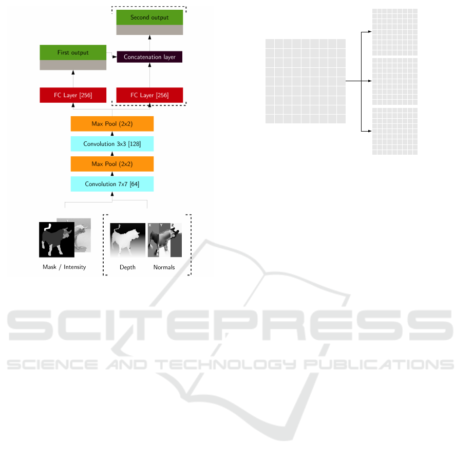
Figure 2: Basic network architecture for the various predic-
tion tasks: The numbers in brackets denote the number of
filters of the convolution layers, the number of nodes of the
fully connected layers (FC layers) or the pooling size of the
pooling stages. Moreover the convolutional modules are la-
beled with the used filter size. The network input consisted
of a 96 × 96 part mask stacked together with the intensity
image and optionally depth and surface normal informa-
tion. For the multi-output models the first network output
is merged into the second output branch. Dotted brackets
indicate optional components of the network that are added
depending on the task.
Following this line of thought it makes sense to be in-
spired by standard architectures for object perception
and to test part recognition performance of different
versions of them.
As basis for each of the perception networks
the ReLU-Conv-Pool network modules suggested by
Krizhevsky et al. (2012) turn out to be a good choice.
The module consists of a 2D-convolutional layer fol-
lowed by a 2D-Maximum-Pooling layer where both
use the recommended ReLU nonlinearity. Following
the approach of Papon and Schoeler (2015) two of
these Conv-Pool modules were stacked with the pa-
rameters of their most successful model. To prevent
from overfitting all layers were adjusted to use the
dropout technique proposed by Hinton et al. (2012).
An overview of the resulting architecture is depicted
in Figure 2.
Figure 3: Illustration of the part ground truth encoding: Part
information is encoded into a matrix with the dimensions of
the input image, where each entry contains the part number
of the corresponding image pixel. Consequently, different
object parts are highlighted by different numbers.
3.2.1 Network Inputs and Preprocessing
The input of the networks are 96× 96 real-valued im-
ages including the intensity information and, option-
ally, depth and surface normal vectors in x-, y- and z-
direction. To ensure standardized inputs all channels
were zero-centered by subtracting the mean across ev-
ery individual feature in the data. Moreover, in or-
der to level the different scales and units the channels
were normalized so that the minimum and maximum
along the dimension is -1 and 1 respectively.
We assume that the object’s parts had been seg-
mented previously and focus our approach on classi-
fying these segmented parts. The part ground truth
is encoded into a matrix having the same size as the
RGB-D image with each entry containing the part
number of the corresponding image pixel. Hereafter
it is referred to as part mask. As illustrated in Fig-
ure 3, the matrix encodes the parent object with a 1,
the part in question with a 2 and the background with
a 0 digit. The network is then requested to predict the
correct label of the part or the area which is designated
with 2. This way, by subsequently masking every un-
classified part with 2, all object parts can be assigned
a label. An overview of all inputs is presented in Fig-
ure 4.
3.2.2 Network Outputs
The network is trained and evaluated in different set-
tings, each predicting different quantities. First, there
is a standard output to predict the eight classes of the
parent objects. Second, there are two more output
modules for part classification: One ’full-part output’,
which predicts each of the 28 parts in the eight parent
object classes; and alternatively, a ’reduced-part out-
VISAPP 2017 - International Conference on Computer Vision Theory and Applications
372

(a) Part mask. (b) Intensity Image.
(c) Depth Image. (d) Surface normals.
Figure 4: Compilation of the different network input types,
which were generated for the training. The part and inten-
sity information is obtained using the Blender graphic en-
gine. The depth channel is generated with the help of the
BlenSor sensor simulation toolbox by Gschwandtner et al.
(2011). Finally, the object surface normals were computed
using the technique presented by Holzer et al. (2012).
put’, which condenses semantically similar parts from
the parent object classes resulting in only 16 distinct
part predictions, e.g. LampesStand and VasesStand
become Stand. In the latter case the output therefore
predicts parts regardless of the actual class of the par-
ent object. Finally, there is an output layer to predict
the rotation angle of the parent object.
Rotation Output. In principle, rotation output can
be realized in two different ways. The obvious possi-
bility is the use of a single output neuron, the activa-
tion value of which represents the predicted rotation
angular. Hereafter this solution is called ’regression
model’. On the other hand it is possible to cast the ro-
tation estimation into a classification task. To achieve
this the possible value range is divided into a number
of small value ranges which are being associated with
a class name. The network is then requested to predict
the correct range. A disadvantage of this approach is
that the network cannot distinguish rotational values
which lie in the same value range. The rotation es-
timation by class is hereafter referred to as ’binned
model’. In contrast to the aforementioned class out-
puts, where the predictions were simply compared to
the correct solution, for the regression output it is nec-
essary to define a proper error metric, e.g. the differ-
ence between predicted and correct value. Evidently,
the maximum possible error in rotation estimation is
180 degree. To reflect this, the error ε
∢
between the
predicted angular α and the actual rotation β is de-
fined as follows:
ε
∢
(α,β) = min(|α− β|, 360− |α− β|) (1)
However, it is important to notice that the use of
this error metric might cause problems in the learn-
ing process. The parameter adjustments of the out-
put neuron depend on the gradient ∇C of the cost
function. In fact, the calculation therefore includes
a derivation with respect to the neuron parameters Θ.
Particularly, if the angular error ε
∢
is used in the cost
function, the neuron output α = σ(x, Θ) with the acti-
vation function σ has to be differentiated:
∇C ∝ ∇ε
∢
(α,β,Θ) ∝ ±
(σ− β)
|σ− β|
· σ
′
The gradient expression then contains the derivation
of the activation function σ
′
(w, b). It is therefore es-
sential to remember that the activation function is a
rectified linear unit. As a result, σ
′
vanishes if its ar-
gument ~w
T
~x+b is smaller than zero. In consequence,
if the weights and the bias adapt to improper values,
∇C vanishes as well and the learning process stops.
To use the regression model it had therefore been
ensured that ~w
T
~x + b is always positive. A simple
way to avoid a vanishing gradient was to initialize the
weights and the bias with w
i
= 0 and b = 90. This way
the training always sets off from ~w
T
~x + b = 90 > 0,
converging safely, even if~x was assigned with an im-
proper value at the beginning of training.
3.3 Training and Testing Methodology
To find optimal learning rates for each training run,
six learning rates between 0.1 and 1 × 10
−6
were
tested. Moreover, the learning rate was automati-
cally reduced if the validation performance stopped
improving (adaptive learning rate). To avoid over-
fitting training was canceled using the early stopping
technique on the validation set.
The separation into training, validation, and test
sets were done as follows: randomly chosen 20% of
the models of each class were excluded from training.
From these models, the test data set with 1000 items
was generated using rotation and scaling. Hence, the
network encounter completely new object instances
in the test. With the 80% remaining object models
the training and validation data sets were generated in
proportion 95% and 5%, respectively.
Each of the generated training examples consists
of a randomly chosen object model placed in the cen-
Part-driven Visual Perception of 3D Objects
373

ter of the scene with random illumination to simu-
late shadow effects. In the first instance the objects
were put to the ground and rotated around the z-axis
to guarantee realistic poses. As the number of in-
stances in each object class differs, an approximately
equal number of scenes for each class has been gener-
ated. This led obviouslyto more frequent occurrences
of object instances of smaller classes throughout the
training. In total, 25 000 scenes were generated as
training set, in which every single object instance oc-
curred at least in 100 different representations.
4 RESULTS AND DISCUSSION
The main focus is here on training and evaluation of
the synthetic data sets in order to achieve a basic un-
derstanding of how well part perception with such a
neural network works.
4.1 Classification
The quantitative results in the following section are
obtained using the test data set containing 1000
scenes with unseen object models, i.e. with object
shapes not seen during training at all.
4.1.1 Classification (Whole Object)
For the first step and to establish a baseline, the convo-
lutional network is trained to predict the eight differ-
ent whole-object classes based on the intensity chan-
nel only (first network output only).
With an overall accuracy of 85.3%, the classifi-
cation proves to be reliable, but it is worth noting
that the performance significantly correlates with the
number of class instances in the data set. While
the perception accuracy of the 44 Guitar instances is
close to perfection (0.97 F1 score) the classification
is less reliable for the Goblets which only counts 12
instances (0.64 F1 score).
4.1.2 Rotation (Whole Object)
As a next step the model is extended with the sec-
ond output to predict the rotation of the whole object
around the z-axis. To measure accuracy for each out-
put the symmetric angular error ε
∢
is calculated as
defined by Equation 1. The Area Under Curve (AUC)
accuracy is calculated as
ε
AUC
= 1−
1
N
N
∑
i
ε
i
∢
180
◦
.
0 20 40 60 80 100 120 140 160 180
Angular error
[
]
0
20
40
60
80
100
Fractional accuracy [%]
Rotation regression: 61.8 %
Binned rotation: 69.5 %
(a) Rotation estimation comparison of binned and regres-
sion model: The binned rotation model outperforms the
rotation model in terms of overall accuracy as well as
share of marginal errors.
0 20 40 60 80 100 120 140 160
180
Angular error
[
]
0
20
40
60
80
100
Fractional accuracy [%]
Chair: 82.6 %
Lampes: 69.3 %
Candelabra: 50.9 %
Guitars: 94.7 %
Goblets: 50.9 %
Vases: 59.4 %
Irons: 60.4 %
Four-legged: 85.2 %
(b) Comparison of the rotation estimation performances
broken down by class: Evidently, a large variation in ac-
curacy is observed ranging from 94.7% for the guitars
class to 50.9% for the goblets class.
Figure 5: Results of the rotation estimation: Following
Gupta et al. (2015), the depiction represents the fraction of
objects for which the model is able to predict the rotation
with an error of less than ε
ϑ
, plotted versus ε
ϑ
.
Using this error metric we find the binned rota-
tion model being able to predict the z-rotation with
an accuracy of 69.5% which clearly outperforms the
rotation regression model by 7.7%. In order to exam-
ine the performance in more detail the representation
by Gupta et al. (2015) is used: It determines the frac-
tion of objects for which the model is able to predict
the rotation with an error less than ε
ϑ
plotting it as
a function of ε
ϑ
. Figure 5a documents the compari-
son of the binned and the regression model using this
representation.
Figure 5a shows that the binned model outper-
forms the regression model: For the binned model
36.8% of all predictions lie under 10
◦
error whereas
this is true for only 11.4% of the regression predic-
VISAPP 2017 - International Conference on Computer Vision Theory and Applications
374

ChairLeg ( 0.98)
ChairSeat ( 0.96)
ChairBack ( 0.99)
LampesHolder ( 0.73)
LampesStand ( 0.74)
LampesLamp ( 0.65)
CandelabraCandle ( 0.92)
CandelabraHandle ( 0.88)
CandelabraFlame ( 0.92)
CandelabraStand ( 0.82)
GuitarsNeck ( 0.99)
GuitarsHead ( 1.00)
GuitarsBody ( 1.00)
GobletsStand ( 0.64)
GobletsHandle ( 0.64)
GobletsContainer ( 0.64)
VasesHandle ( 0.73)
VasesStand ( 0.58)
VasesHead ( 0.59)
VasesContainer ( 0.81)
IronsHandle ( 0.75)
IronsBody ( 0.82)
IronsIron ( 0.68)
Four-leggedBody ( 0.82)
Four-leggedEars ( 0.81)
Four-leggedHead ( 0.92)
Four-leggedLeg ( 0.97)
Four-leggedTail ( 0.81)
Predicted (F1 score)
Four-leggedTail
Four-leggedLeg
Four-leggedHead
Four-leggedEars
Four-leggedBody
IronsIron
IronsBody
IronsHandle
VasesContainer
VasesHead
VasesStand
VasesHandle
GobletsContainer
GobletsHandle
GobletsStand
GuitarsBody
GuitarsHead
GuitarsNeck
CandelabraStand
CandelabraFlame
CandelabraHandle
CandelabraCandle
LampesLamp
LampesStand
LampesHolder
ChairBack
ChairSeat
ChairLeg
Actual class
0 0 0 0 0 0 0 0 0 0 0 0 0 0 0 0 0 0 0 0 0 0 0 1 13 2 0 66
0 0 0 0 0 0 0 0 0 0 0 0 0 0 0 0 0 0 0 0 0 0 0 0 0 0
111 0
0 0 0 0 0 0 0 0 0 0 0 0 0 0 0 0 0 1 0 0 0 0 0 3 1
102 3 1
0 1 0 0 0 0 0 0 0 0 0 0 0 0 0 0 0 0 0 0 0 0 0 0
102 3 0 5
0 0 0 0 0 0 0 0 0 0 0 0 0 0 0 0 0 0 0 0 0 0 0
111 0 0 0 0
0 3 0 0 0 0 0 0 0 5 0 0 0 0 0 0 2 0 0 0 0 3 39 6 0 3 0 1
0 6 0 0 0 0 0 0 0 1 0 0 0 0 0 0 0 0 0 3 22
91 2 2 0 0 0 0
0 0 0 0 0 0 0 10 0 0 0 0 0 0 0 0 0 0 15 0
92 0 0 0 10 0 0 0
0 0 0 0 0 10 0 0 0 17 0 0 0 0 0 0 0 0 0
94 0 0 0 5 0 0 0 0
0 0 0 1 0 0 0 3 3 0 0 0 0 0 0 0 5 14 79 8 2 0 0 11 0 0 0 0
0 0 0 0 12 0 0 3 3 0 0 0 0 0 0 0 24 58 25 0 0 1 0 0 0 0 0 0
0 0 1 2 0 4 1 4 0 0 2 0 0 0 0 0
91 0 19 0 2 0 0 0 0 0 0 0
0 0 0 0 0 64 0 0 0 0 0 0 0 0 0 56 0 0 0 0 0 0 0 0 0 0 0 0
0 0 0 64 0 0 0 0 0 0 0 0 0 0 56 0 0 0 0 0 0 0 0 0 0 0 0 0
0 0 0 0 64 0 0 0 0 0 0 0 0 56 0 0 0 0 0 0 0 0 0 0 0 0 0 0
0 0 0 0 0 0 0 0 0 0 0 0
142 0 0 0 0 0 0 0 0 0 0 0 0 0 0 0
0 0 0 0 0 0 0 0 0 0 0
142 0 0 0 0 0 0 0 0 0 0 0 0 0 0 0 0
0 0 0 0 0 0 0 0 0 0
142 0 0 0 0 0 0 0 0 0 0 0 0 0 0 0 0 0
0 0 0 0 9 0 0 0 0
102 0 0 0 0 0 0 0 0 0 0 0 0 12 0 0 0 0 0
0 0 0 0 0 0 0 0
110 0 0 0 0 0 0 0 0 0 0 0 0 0 0 0 13 0 0 0
0 0 0 3 0 0 0
113 0 0 0 0 0 0 0 0 0 0 0 0 0 0 0 0 1 0 0 6
0 0 0 0 0 11
108 0 0 0 0 0 0 0 0 0 0 0 0 0 0 0 0 4 0 0 0 0
0 1 0 1 0
105 2 0 0 0 0 0 0 0 0 0 0 0 0 0 0 0 0 16 0 0 0 0
0 0 0 0
123 0 0 0 0 2 0 0 0 0 0 0 0 0 0 0 0 0 0 0 0 0 0 0
0 0 1
113 0 5 0 0 1 0 0 1 0 0 0 0 0 0 3 0 0 0 0 0 0 0 0 1
0 0
126 0 0 0 0 0 0 0 0 0 0 0 0 0 0 0 0 0 0 0 0 0 0 0 0 0
0
126 0 0 0 0 0 0 0 0 0 0 0 0 0 0 0 0 0 0 0 0 0 0 0 0 0 0
122 0 0 0 0 0 0 0 0 0 0 0 0 0 0 0 0 0 0 0 0 0 0 0 0 0 4 0
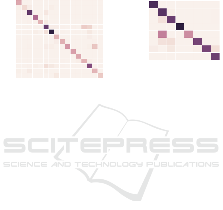
Overall accuracy: 82.3 %
Figure 6: Confusion matrix of the full part prediction model, which is trained on the part mask channel. The network is able
to predict parts without major problems but tends to confuse both vases’ and goblets’ components.
tions. Moreover it is obvious that for a significant
fraction of predictions the angular error is greater than
100
◦
and therefore not usable in a real world applica-
tion.
Examining the rotational estimation for each ob-
ject class, we find that for both models the accuracy
rates are not homogeneous. In fact, as presented in
Figure 5b, rates vary from 94.7% in Guitars class to
50.9% in the Goblets class with 83.8% to 5.8% under
10
◦
error, respectively. The scores correlate with the
number of different object instances within classes.
The per-class analysis also discloses that for the three
classes Guitars, Four-legged and Chairs, the rotation
estimation is reliable in the sense that more than 75%
of all predictions have an error less than 25
◦
.
Motivated by these results all of the following
simulations (if not stated otherwise) are performed us-
ing the binned rotational estimation.
4.1.3 Part Recognition
First, the network is trained to predict the full part
label, which contains the parent object’s class name,
e.g. VasesContainer contains Vases. For this only the
two-dimensional part masks are used as input. This
method achieved an overall classification accuracy of
82.3%. The corresponding confusion matrix is docu-
mented in Figure 6.
The performance for different parts varies in a
noteworthy manner ranging from 53% for Lampes-
Lamp up to even 100% for GuitarsBody. Notably the
network tended to confuse Goblet parts with Lamp
parts and had problems keeping the parts of Vases -
Handle, Stand - apart. In particular, in half of all
classes an accuracy of over 90% is achieved, while
the Goblet part classification falls under 50%.
One remarkable observation is that the network
confuses GobletsStand with LampesStand and also
GobletsHandle with LampesHolder in roughly one
half of the predictions performed on these classes.
These findings suggest that the network recognized
semantic part features, e.g. Stands and Handles,
rather than the class of the parent object and its parts.
Therefore it seems reasonable to train a network for
these particular part classes. As Stands and Handles
are not part in all of the eight parent object classes,
this part-focused classification consequently reduces
the number of classes, hence it is called reduced part
classification. Experiments indicate that employing
such a reduced classification model turned out to be
Part-driven Visual Perception of 3D Objects
375
Seat ( 0.96)
Iron ( 0.79)
Body ( 0.94)
Leg ( 0.98)
Candle ( 0.92)
Handle ( 0.74)
Stand ( 0.90)
Ears ( 0.80)
Flame ( 0.92)
Container ( 0.77)
Neck ( 0.99)
Back ( 0.98)
Holder ( 0.72)
Head ( 0.80)
Lamp ( 0.68)
Tail ( 0.86)
Predicted (F1 score)
Tail
Lamp
Head
Holder
Back
Neck
Container
Flame
Ears
Stand
Handle
Candle
Leg
Body
Iron
Seat
Actual class
0 0 0 0 0 0 0 14 0 0 0 0 0 1 0 67
4 0 12 0 0 4 0 0 0 0 0 0 1 0 104 0
0 0 3 5 0 33 17 6 2 0 0 0 0
311 0 2
0 0 0 0 1 2 0 0 2 0 0 6 107 6 1 0
0 0 0 0 0 0 0 0 0 0 0 126 0 0 0 0
0 0 0 0 0 0 0 0 0 0 142 0 0 0 0 0
0 0 2 0 0 7 6 0 0 153 0 0 0 4 74 0
0 0 0 0 0 0 0 9 111 0 0 0 0 0 3 0
1 0 0 0 0 0 0 100 0 0 0 0 0 8 0 2
0 1 0 6 0 31
438 0 2 0 0 0 0 16 0 0
0 0 0 0 1
355 8 9 2 0 2 0 65 51 0 3
0 0 3 0 106 14 0 0 0 0 0 0 0 0 0 0
0 0 0 237 0 0 0 0 0 0 0 0 0 0 0 0
1 0
359 0 0 19 1 0 0 0 0 0 0 0 0 0
5 41 8 1 0 0 6 0 0 0 0 0 0 1 0 0
126 0 0 0 0 0 0 0 0 0 0 0 0 0 0 0
Overall accuracy: 85.4 %
Figure 7: Confusion matrix of the reduced part classifica-
tion carried out by a network trained on the part mask input
channel only. Problems occurred only in the prediction of
handle and container parts.
a reasonable choice. The overall accuracy of the re-
duced part perception lies at 85.4% and, therefore,
on the same scale as the full class part recognition.
The rates ranged from 62% for the Holder class to
92% for the Seat class. Remarkably, like the full
model, the reduced one confuses the Handle with
Holder, with both part classes having the same func-
tion. It is not possible to compare the scores of the
full and reduced models in a direct manner since the
16-reduced-classes identification task is easier than
that for the 28-full-classes problem. Nevertheless, the
good accuracy of the reduced model supports the pre-
sumption that the network is able to identify parts re-
gardless of the parent object class.
4.1.4 Part-driven Object Classification
Provided with the correctly classified parts, it might
be possible to derive the class name of the parent ob-
ject. Next, we investigate if this procedure leads to
a better performance compared to directly predicting
the object class. To realize such a part-driven object
classification, the object in question has to be seg-
mented into parts, which then themselves are classi-
fied. From the resulting part labels the parent object
class is inferred. For example, if the part classifica-
tion yields ChairSeat, LampesStand and ChairBack it
is likely that the parent object is a Chair. This tech-
nique is implemented for all models with part recog-
nition which did not provide a class output natively.
For the part recognition model the mask input was
Chair(0.98)
Lampes(0.74)
Candelabra(0.89)
Guitars(1.00)
Goblets(0.64)
Vases(0.91)
Irons(0.91)
Four-legged(0.95)
Predicted(F1 score)
Four-legged(20)
Irons(18)
Vases(28)
Goblets(12)
Guitars(44)
Candelabra(28)
Lampes(20)
Chair(20)
Actual class
(Instance count)
0 0 0 0 0 0 0 111
3 0 6 0 0 2 106 10
0 9 10 0 0
107 0 0
0
64 0 0 56 0 0 0
0 0 0
142 0 0 0 0
0 9
113 0 0 0 0 1
1
121 2 0 0 0 0 1
126 0 0 0 0 0 0 0
Overall accuracy: 88.2%
Figure 8: Confusion matrix of the COSEG object classifi-
cation, which was derived from the recognized part. The
method tends to confuse lampes with goblets but outper-
forms the standard classification model, which was trained
to recognize the objects as-a-whole.
used as discussed in the previous section. This leads
to a classification accuracy of 88.2%. Figure 8 shows
the corresponding confusion matrix. Compared to the
original, direct classification model, which uses inten-
sity information and is only and explicitly trained for
object classification, this is an improvement of 2.9%.
The fact that objects can be recognized just from their
parts using CNN could be considered an important
observation.
5 CONCLUSIONS AND FUTURE
WORK
The presented work provesthat it is possible to realize
part perception of everyday objects with synthetically
trained deep neural networks. Two aspects are po-
tentially of more far reaching interest. 1) We showed
that parts are recognized independently of their par-
ent object class. This kind of generalization is a typ-
ical human trait. For us a leg remains a leg whether
it comes from a chair or a table. 2) We could also
demonstrate that object recognition can be achieved
from recognizing part combinations from which the
object class is then inferred. Here, we found that for
our system part-drivenobject classification, where the
parent object class is derived from the object parts,
outperformed a comparable standard object classifi-
cation network which does not use object parts as an
intermediate representation.
VISAPP 2017 - International Conference on Computer Vision Theory and Applications
376

In our future work, we plan to test the part-based
perception approach on a bigger data set also using
more advanced network structures as well as extend
the approach to infer not only objects, but also their
functions (affordances). The method performance
will be compared to the existing techniques and vali-
dated on real RGB-D data. In order to make predic-
tions more robust, more rotation axes and view angles
could be included in the training. Additionally, artifi-
cial noise and visual obstacles could be applied on the
training data to increase robustness even further.
REFERENCES
Biederman, I. (1987). Recognition-by-components: a the-
ory of human image understanding. Psychological re-
view, 94(2):115.
Chen, X., Golovinskiy, A., and Funkhouser, T. (2009). A
benchmark for 3D mesh segmentation. ACM Trans-
actions on Graphics (Proc. SIGGRAPH), 28(3).
Felzenszwalb, P. F., Girshick, R. B., McAllester, D., and
Ramanan, D. (2010). Object detection with discrimi-
natively trained part-based models. IEEE transactions
on pattern analysis and machine intelligence, 32(9).
Girshick, R., Donahue, J., Darrell, T., and Malik, J. (2014).
Rich feature hierarchies for accurate object detection
and semantic segmentation. In IEEE Conference on
Computer Vision and Pattern Recognition (CVPR),
pages 580–587. IEEE.
Gschwandtner, M., Kwitt, R., Uhl, A., and Pree, W. (2011).
Blensor: Blender sensor simulation toolbox. In Ad-
vances in Visual Computing, volume 6939 of Lec-
ture Notes in Computer Science, chapter 20. Springer
Berlin / Heidelberg, Berlin, Heidelberg.
Gupta, S., Arbel´aez, P., Girshick, R., and Malik, J. (2015).
Aligning 3d models to rgb-d images of cluttered
scenes. In Proceedings of the IEEE Conference
on Computer Vision and Pattern Recognition, pages
4731–4740.
Hinton, G. E., Srivastava, N., Krizhevsky, A., Sutskever, I.,
and Salakhutdinov, R. R. (2012). Improving neural
networks by preventing co-adaptation of feature de-
tectors. arXiv preprint arXiv:1207.0580.
Holzer, S., Rusu, R. B., Dixon, M., Gedikli, S., and Navab,
N. (2012). Adaptive neighborhood selection for real-
time surface normal estimation from organized point
cloud data using integral images. In International
Conference on Intelligent Robots and Systems (IROS),
pages 2684–2689. IEEE.
Krizhevsky, A., Sutskever, I., and Hinton, G. E. (2012). Im-
agenet classification with deep convolutional neural
networks. In Advances in neural information process-
ing systems, pages 1097–1105.
Leibe, B., Leonardis, A., and Schiele, B. (2004). Combined
object categorization and segmentation with an im-
plicit shape model. In Workshop on statistical learn-
ing in computer vision, ECCV, volume 2.
Oliveira, G. L., Valada, A., Bollen, C., Burgard, W., and
Brox, T. (2016). Deep learning for human part dis-
covery in images. In IEEE International Conference
on Robotics and Automation (ICRA).
Papon, J. and Schoeler, M. (2015). Semantic pose using
deep networks trained on synthetic rgb-d. In IEEE
International Conference on Computer Vision (ICCV).
Schoeler, M., Papon, J., and Worgotter, F. (2015). Con-
strained planar cuts - object partitioning for point
clouds. In The IEEE Conference on Computer Vision
and Pattern Recognition (CVPR).
Tsogkas, S., Kokkinos, I., Papandreou, G., and Vedaldi, A.
(2015). Semantic part segmentation with deep learn-
ing. arXiv preprint arXiv:1505.02438.
Wang, Y., Asafi, S., van Kaick, O., Zhang, H., Cohen-Or,
D., and Chen, B. (2012). Active co-analysis of a set
of shapes. 31(6):165:1–165:10.
Zhang, N., Donahue, J., Girshick, R., and Darrell, T.
(2014). Part-based r-cnns for fine-grained category de-
tection. In European Conference on Computer Vision.
Springer.
Part-driven Visual Perception of 3D Objects
377
