Generative vs. Discriminative Deep Belief Netwok for 3D Object
Categorization
Nabila Zrira
1
, Mohamed Hannat
1
, El Houssine Bouyakhf
1
and Haris Ahmad Khan
2,3
1
LIMIARF Laboratory, Mohammed V University Rabat, Faculty of Sciences, Rabat, Morocco
2
Le2i, UMR CNRS 6306, Arts et M
´
etiers, Univ. Bourgogne Franche-Comt
´
e, Dijon, France
3
NTNU, Norwegian University of Science and Technology, Gjøvik, Norway
Keywords:
3D Object Categorization, Point Clouds, Viewpoint Feature Histogram (VFH), DDBN, GDBN, RBM, Joint
Density Model, Bback-propagation.
Abstract:
Object categorization has been an important task of computer vision research in recent years. In this paper, we
propose a new approach for representing and learning 3D object categories. First, We extract the Viewpoint
Feature Histogram (VFH) descriptor from point clouds and then we learn the resulting features using deep
learning architectures. We evaluate the performance of both generative and discriminative deep belief network
architectures (GDBN/DDBN) for object categorization task. GDBN trains a sequence of Restricted Boltzmann
Machines (RBMs) while DDBN uses a new deep architecture based on RBMs and the joint density model.
Our results show the power of discriminative model for object categorization and outperform state-of-the-art
approaches when tested on the Washington RGBD dataset.
1 INTRODUCTION
With the advent of new 3D sensors like Microsoft
Kinect, 3D perception became a fundamental vision
research in mobile robotic applications like scene
manipulation or grasping, scene understanding, and
3D point cloud classification. The Point Cloud Li-
brary (PCL) was developed by Rusu et al. (Rusu
and Cousins, 2011) in 2010 and was officially pub-
lished in 2011. This open source library, licensed
under Berkeley Software Distribution (BSD) terms,
represents a collection of state-of-the-art algorithms
and tools that operate with 3D point clouds. Sev-
eral studies have been made based on PCL detectors
and descriptors, allowing for 3D object recognition
applications. PCL integrates several 3D detectors as
well as 3D local and global descriptors. In 3D local
descriptors, each point is described by its local ge-
ometry. They are developed for specific applications
such as object recognition, and local surface catego-
rization. This local category includes Signature of
Histograms of OrienTation (SHOT) (Tombari et al.,
2010), Point Feature Histograms (PFH) (Rusu et al.,
), Fast Point Feature Histograms (FPFH) (Rusu et al.,
2009), SHOTCOLOR (Tombari et al., 2011), and so
on. On the other hand, the 3D global descriptors de-
scribe object geometry and they are not computed for
individual points, but for a whole cluster instead. The
global descriptors are high-dimensional representa-
tions of object geometry. They are usually calculated
for subsets of the point clouds that are likely to be ob-
jects. The global category encodes only the shape in-
formation and includes Viewpoint Feature Histogram
(VFH) (Rusu et al., 2010), Clustered Viewpoint Fea-
ture Histogram (CVFH) (Aldoma et al., 2011), CVFH
(OUR-CVFH) (Aldoma et al., 2012), and Ensemble
of Shape Functions (ESF) (Wohlkinger and Vincze,
2011).
The ability to identify or recognize 3D objects
is highly valuable for performing imperative tasks in
mobile robotics. Machine learning techniques are ap-
plied for this task which include Support Vector Ma-
chines (SVMs) (LeCun et al., 2004) (Zhang et al.,
2006) (Janoch et al., 2013), Nearest Neighbor (NN)
(McCann and Lowe, 2012), Hidden Markov Model
(HMM) (Torralba et al., 2003), and Artificial Neural
Network (ANN) (Basu et al., 2010).
The origin of ANN dates back to efforts for find-
ing a mathematical representation for information
processing in human brains. The brain consists of a
large number of processing units (10
11
units accord-
ing to (Azevedo et al., 2009)) which operate in paral-
lel and are highly inter-connected. ANN are designed
in a similar manner using a large number of process-
98
Zrira N., Hannat M., Bouyakhf E. and Ahmad khan H.
Generative vs. Discriminative Deep Belief Netwok for 3D Object Categorization.
DOI: 10.5220/0006151100980107
In Proceedings of the 12th International Joint Conference on Computer Vision, Imaging and Computer Graphics Theory and Applications (VISIGRAPP 2017), pages 98-107
ISBN: 978-989-758-226-4
Copyright
c
 2017 by SCITEPRESS – Science and Technology Publications, Lda. All rights reserved

ing units called perceptrons that operate in the parallel
process. Research on ANN discover some limitations
of the capability of perceptrons and invent multilayer
perceptron (MLP) neural networks (Rumelbart and
McClelland, 1986). Unfortunately, MLP also shows
the limitations for some complex nonlinear functions
that cannot be efficiently represented by this type of
networks. In (Serre et al., 2007), authors show the
evidence that the brain of a mammal is organized in
the form of a deep architecture. A specified input is
characterized at various levels of abstraction, where
every level relates to a diverse area of cortex. Re-
searchers used the deep architecture concept in neu-
ral networks for training new deep multi-layer neural
networks which are stimulated by the biological depth
of brain. Such deep models involve numerous layers
and parameters that require learning through the com-
plex process. To deal with this problem, the authors
in (Hinton et al., 2006a) suggest a deep belief network
(DBN) with multiple layers of hidden units.
DBN is a graphical model consisting of undirected
networks at the top hidden layers and directed net-
works in the lower layers. The learning algorithm
uses greedy layer-wise training by stacking restricted
Boltzmann machines (RBM) which contain hidden
layer for modeling the probability distribution of per-
ceptible variables. The idea of having multiple hid-
den layers is that the preceding hidden layer acts as
the visible layer for the next hidden layer and thus the
model can incrementally learn more complex features
of data.
In general, deep learning architectures can be
broadly classified into three main categories (Deng,
2014):
1. Generative deep architectures: the aim is to char-
acterize the high-order correlation properties of
the visible data for pattern analysis or synthesis
purposes, and/or characterize the joint statistical
distributions of the visible data and their associ-
ated classes;
2. Discriminative deep architectures: the aim is to
directly provide discriminative power for pattern
classification, often by characterizing the poste-
rior distributions of classes conditioned on the vis-
ible data;
3. Hybrid deep architectures: the aim is to com-
bine the power of discrimination with the outputs
of generative architectures via better optimization
or/and regularization.
Our work focuses on 3D object categorization for
mobile robotic grasping. First, we extract Viewpoint
Feature Histogram (VFH) descriptors that encode ge-
ometric features of 3D point clouds followed by learn-
ing the resulting features using effective deep archi-
tectures. We evaluate both generative and discrimina-
tive deep belief network (GDBN/DDBN) using dif-
ferent RBM training techniques which include Con-
trastive Divergence (CD), Persistent Contrastive Di-
vergence (PCD), and Free Energy in Persistent Con-
trastive Divergence (FEPCD).
The main contributions of our paper are:
• We propose a new 3D object categorization
pipeline based on VFH descriptor and deep learn-
ing architectures;
• We compare the extracted features with GDBN
and DDBN architectures in order to show the
difference between generative and discriminative
models for object categorization.
The rest of the paper is organized as follows. In Sec-
tion 2 we review previous works. In Section 3 we give
a brief description of VFH descriptor. In Section 4
we present an overview of our proposed approach. In
Section 5 two different deep learning architectures are
illustrated. And in Section 6, the experimental results
carried out to demonstrate the functionality and us-
ability of this work are presented. Finally, in Section
7 the main conclusions and future works are outlined.
2 PREVIOUS WORK
Most of the recent work on 3D object categoriza-
tion have focused on appearance, shapes, and Bag of
Words (BoW) extracted from certain viewing point
changes of the 3D objects. In (Toldo et al., 2009),
authors introduce Bag of Words (BoW) approach for
3D object categorization. They use spectral cluster-
ing to select seed-regions then compute the geometric
features of the object sub-parts. Vector quantization is
applied to these features in order to obtain BoW his-
tograms for each mesh. Finally, Support Vector Ma-
chine is used to classify different BoW histograms for
3D objects. In (Nair and Hinton, 2009), a top-level
model of Deep Belief Networks (DBNs) is presented
for 3D object recognition. This model is a third-order
Boltzmann machine that is trained using a combina-
tion of both generative and discriminative gradients.
The model performance is evaluated on NORB im-
ages where the dimensionality for each stereo-pair
image is reduced by using a foveal image. The final
representation consists of 8976-dimensional vectors
that are learned with a top-level model for Deep Belief
Nets (DBN). In (Bo et al., 2011), a set of kernel fea-
tures is introduced for object recognition. The authors
develop kernel descriptors on depth maps that model
Generative vs. Discriminative Deep Belief Netwok for 3D Object Categorization
99

size, depth edges, and 3D shape. The main match ker-
nel framework defines pixel attributes, designs match
kernels in order to measure the similarities of image
patches and then determines low dimensional match
kernels. In (Lai et al., 2011a), the authors build a
new RGBD dataset and propose methods to recognize
and detect RGBD objects. They use SIFT descriptor
to extract visual features and spin image descriptor
to extract shape features that are used for computing
efficient match kernel (EKM). Finally, linear support
vector (LiSVM), gaussian kernel support vector ma-
chine (kSVM) and random forest (RF) are trained to
recognize both the category and the instance of ob-
jects. In (Madry et al., 2012), the authors propose
the Global Structure Histogram (GSH) in order to
describe the point cloud information. The approach
encodes the structure of local feature response on a
coarse global scale to retain low local variations and
keep the advantage of global representativeness. GSH
can be instantiated in partial object views and learned
using complete or incomplete information about an
object. In (Socher et al., 2012), the authors intro-
duce the first convolutional-recursive deep learning
model for 3D object recognition. They compute a sin-
gle CNN layer to extract low-level features from both
color and depth images. Then, these representations
are provided as input to a set of RNNs with random
weights that produce high-quality features. Finally,
The concatenation of all the resulting vectors forms
the final feature vector for a softmax classifier. The
authors in (Schwarz et al., 2015) develop a meaning-
ful feature set that results from the pre-trained stage of
Convolutional Neural Network (CNN). The depth and
RGB images are processed independently by CNN
and the resulting features are then concatenated to de-
termine the category, instance, and pose of the ob-
ject. In (Alexandre, 2016), author proposes a new
approach for RGBD object classification. Four inde-
pendent Convolutional Neural Networks (CNNs) are
trained, one for each depth data and three for RGB
data and then trains these CNNs in a sequence. The
decisions of each network are combined to obtain the
final classification result. The authors of (Ouadiay
et al., 2016) propose a new approach for real 3D ob-
ject recognition and categorization using Deep Belief
Networks. First, they extract 3D keypoints from point
clouds using 3D SIFT detector and then they com-
pute SHOT/SHOTCOLOR descriptors. The perfor-
mance of the approach is evaluated on two datasets:
Washington RGBD object dataset and real 3D object
dataset.
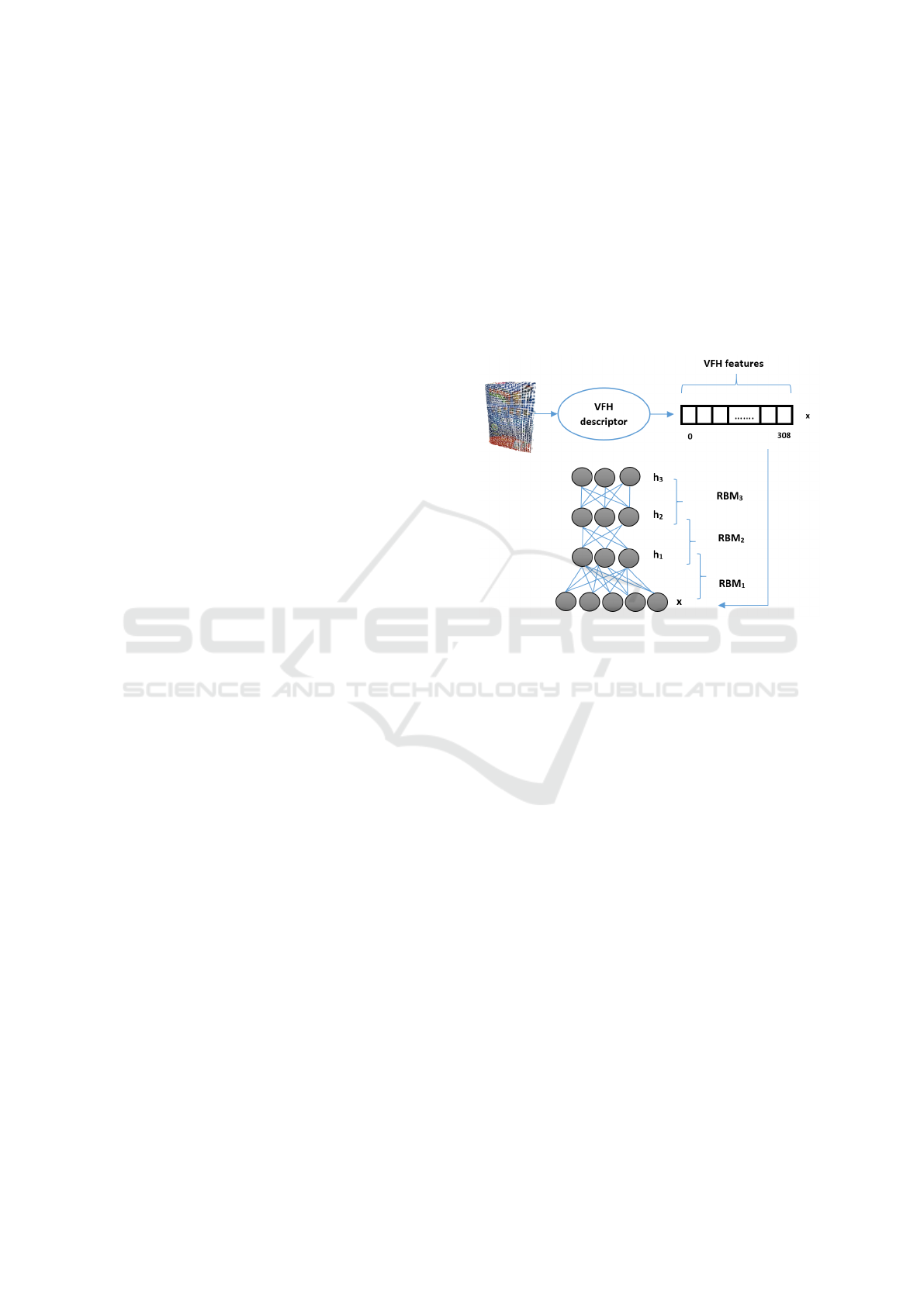
3 METHOD OVERVIEW
In this work, we use the VFH descriptor to describe
the set of 3D point clouds and then we extract the
geometric features which are considered as the input
layer x of GDBN and DDBN architectures. The input
layer has a number N of units which is equivalent to
the quantity of sample data x (308). Finally, we fix
three hidden layers in both GDBN and DDBN archi-
tectures. Figure 1 summarizes the main steps of our
approach.
Figure 1: Our proposed approach for 3D object categoriza-
tion.
The general approach is achieved as follows:
1. Extract geometric features for all training set us-
ing VFH descriptor;
2. Input layer x takes the extracted geometric fea-
tures;
3. Train RBMs using CD, PCD or FEPCD training
(see Section 5.3):
• training the first RBM;
• training the second RBM using the training data
resulting from the first RBM learning;
• training the third RBM: for GDBN architecture,
RBM is generative. Whereas for DDBN archi-
tecture, we train a joint density model through
discriminative RBM and then each conceivable
label is tested with a test vector. The label
which contains the least energy is selected as
the best corresponding class.
4. Use the back-propagation technique through the
whole classifier to fine-tune the weights for an op-
timal classification.
VISAPP 2017 - International Conference on Computer Vision Theory and Applications
100

4 POINT CLOUD PROCESSING
4.1 Point Clouds
The point cloud is a data structure which represents
three-dimensional data. In 3D cloud, the points are
usually described by their x, y and z geometric coor-
dinates of a sampled surface. When the point cloud
contains the color information, the structure becomes
four-dimensional data. Point clouds can be obtained
using stereo cameras, 3D laser scanners, Time-of-
flight cameras or Kinect.
In 3D space, points are defined in a clockwise ref-
erence frame that is centered at the intersection of the
optical axis with the plane which contains the front
wall of the camera. The reference frame is decom-
posed as follows:
• x-axis: is horizontal and directed to the left;
• y-axis: is vertical and faces up;
• z-axis: coincides with the optical axis of the cam-
era. It is turned towards the object.
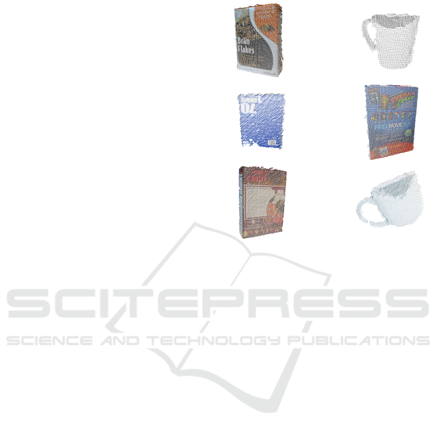
4.2 Washington RGBD Dataset
Washington RGBD dataset is a large dataset built
for 3D object recognition and categorization applica-
tions. It is a collection of 300 common household
objects which are organized into 51 categories. Each
object is placed on a turntable and is captured for
one whole rotation in order to obtain all object views
using Kinect camera that records synchronized and
aligned 640x480 RGB and depth images at 30 Hz (Lai
et al., 2011b).
4.3 Viewpoint Feature Histogram
(VFH)
The global descriptors are high-dimensional represen-
tations of object geometry. They are more efficient
in object recognition, geometric categorization, and
shape retrieval. Global descriptors describe object ge-
ometry. They are not computed for individual points,
but for a whole cluster.
The viewpoint feature histogram (VFH) (Rusu
et al., 2010) computes a global descriptor of the point
cloud and consists of two components:
1. a surface shape component;
2. a viewpoint direction component.
VFH aims to combine the viewpoint direction di-
rectly into the relative normal angle calculation in the
FPFH descriptor (Rusu et al., 2009). The viewpoint-
dependent component of the descriptor is a histogram
Figure 2: A sample of selected point clouds from Washing-
ton RGBD dataset.
of the angles between the vector (p
c
− p
v
) and each
point’s normal. This component is binned into a 128-
bin histogram. The other component is a simplified
point feature histogram (SPFH) estimated for the cen-
troid of the point cloud and an additional histogram of
distances of all points in the cloud to the cloud’s cen-
troid.
The three angles (α, φ, θ) with the distance d be-
tween each point and the centroid are binned into a
45-bin histogram. The total length of VFH descrip-
tor is the combination of these two histograms and is
equal to 308 bins.
5 DEEP LEARNING
ARCHITECTURES
In this section, we briefly introduce both Gen-
erative and Discriminative Deep Belief Network
(GDBN/DDBN) architectures. We also illustrate the
difference between the Generative and Discrimina-
tive restricted Boltzmann machine (GRBM/DRBM)
which constitute many layers in DBN architecture.
Generative vs. Discriminative Deep Belief Netwok for 3D Object Categorization
101

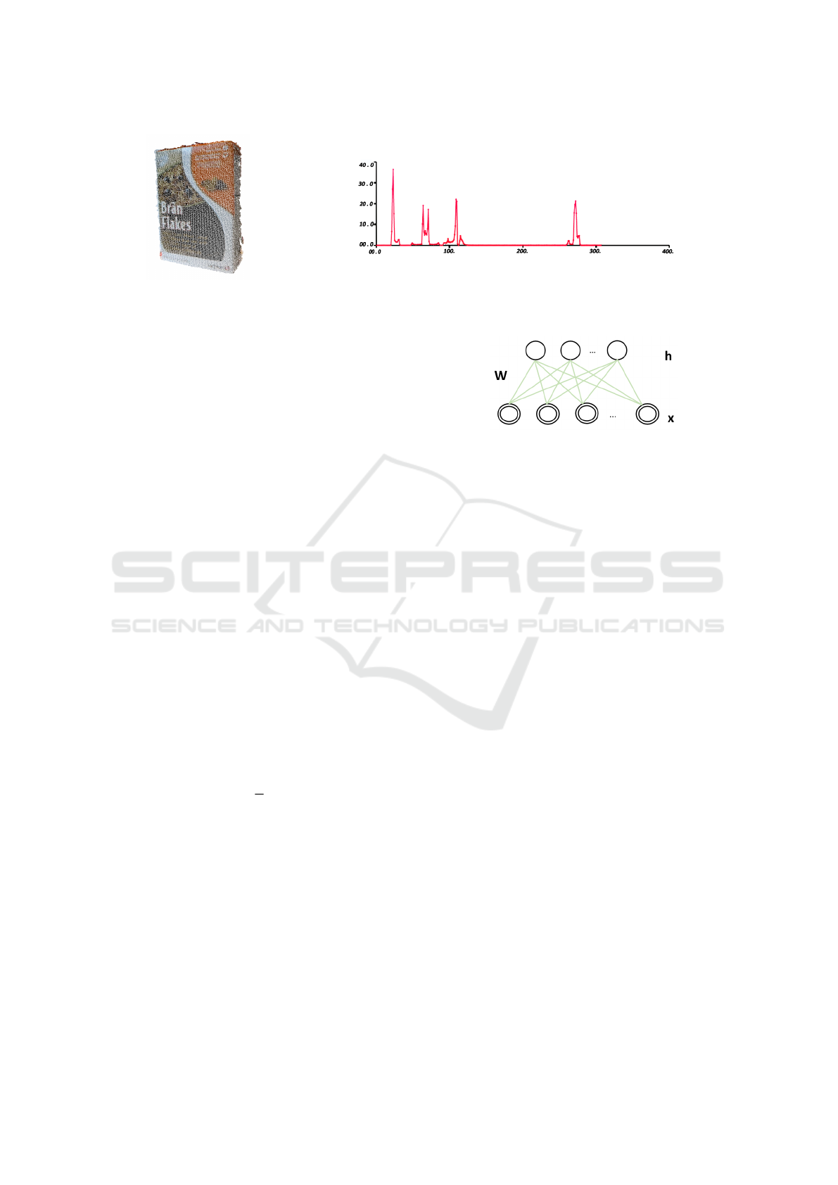
Figure 3: (a) 3D point cloud of food box. (b) VFH descriptor of food box point cloud: x-axis represents a number of histogram
bin and y-axis represents a percentage of points falling in each bin.
5.1 Generative Deep Belief Network
(GDBN)
5.1.1 Restricted Boltzmann Machines (RBMs)
Restricted Boltzmann Machines (RBMs) (Smolensky,
1986) are a specific category of energy based model
which include hidden variables. RBMs are restricted
in the sense so that no hidden-hidden or variable-
variable connections exist. The architecture of a gen-
erative RBM is illustrated in Figure 4.
RBMs are a parameterized generative stochastic
neural network which contain stochastic binary units
on two layers: the visible layer and the hidden layer.
1. Visible units (the first layer): they contain visible
units (x) that correspond to the components of an
observation (i.e. VFH descriptors in this case of
study);
2. Hidden units (the second layer): they contain hid-
den units (h) that model dependencies between
the components of observations.
The stochastic nature of RBMs results from the
fact that the visible and hidden units are stochastic.
The units are binary, i.e. x
i
,h
j
∈ {0, 1}∀ i and j, and
the joint probability which characterize the RBM con-
figuration is the Boltzmann distribution:
p(x,h) =
1
Z
e
−E(x,h)
(1)
The normalization constant is Z =
∑
x,h
e
−E(x,h)
and the energy function of an RBM is defined as:
E(x,h) = −b
0
x − c
0
h − h
0
W x (2)
where:
• W represents the symmetric interaction term be-
tween visible units (x) and hidden units (h);
• b and c are vectors that store the visible (input)
and hidden biases (respectively).
RBMs are proposed as building blocks of multi-
layer learning deep architectures called deep belief
Figure 4: Generative RBM model. The visible units x and
hidden units h are connected through undirected and sym-
metric connections. There are no intra-layer connections.
networks. The idea behind is that the hidden neu-
rons extract pertinent features from the visible neu-
rons. These features can work as the input to another
RBM. By stacking RBMs in this way, the model can
learn features for a high-level representation.
5.1.2 GDBN Architecture
Deep Belief Network (DBN) is the probabilistic gen-
erative model with many layers of stochastic and hid-
den variables. In (Hinton et al., 2006b), the authors
introduce the motivation for using a deep network ver-
sus a single hidden layer (i.e. a DBN vs. an RBM).
The power of deep networks is achieved by having
more hidden layers. However, one of the major prob-
lems for training deep network is how to initialize the
weights W between the units of two consecutive lay-
ers ( j − 1 and j), and the bias b of layer j. Random
initializations of these parameters can cause poor lo-
cal minima of the error function resulting in low gen-
eralization. For this reason, Hinton et al. introduced
a DBN architecture based on training sequence of
RBMs. DBN train sequentially as many RBMs as the
number of hidden layers that constitute its architec-
ture, i.e for a DBN architecture with l hidden layers,
the model has to train l RBMs. For the first RBM,
the inputs consist of the DBN’s input layer (visible
units) and the first hidden layer. For the second RBM,
the inputs consist of the hidden unit activations of the
previous RBM and the second hidden layer. The same
holds for the remaining RBMs to browse through the l
layers. After the model performs this layer-wise algo-
VISAPP 2017 - International Conference on Computer Vision Theory and Applications
102

rithm, a good initialization of the biases and the hid-
den weights of the DBN is obtained. At this stage,
the model should determine the weights from the last
hidden layer for the outputs. To obtain a successfully
supervised learning, the model ”fine-tunes” the result-
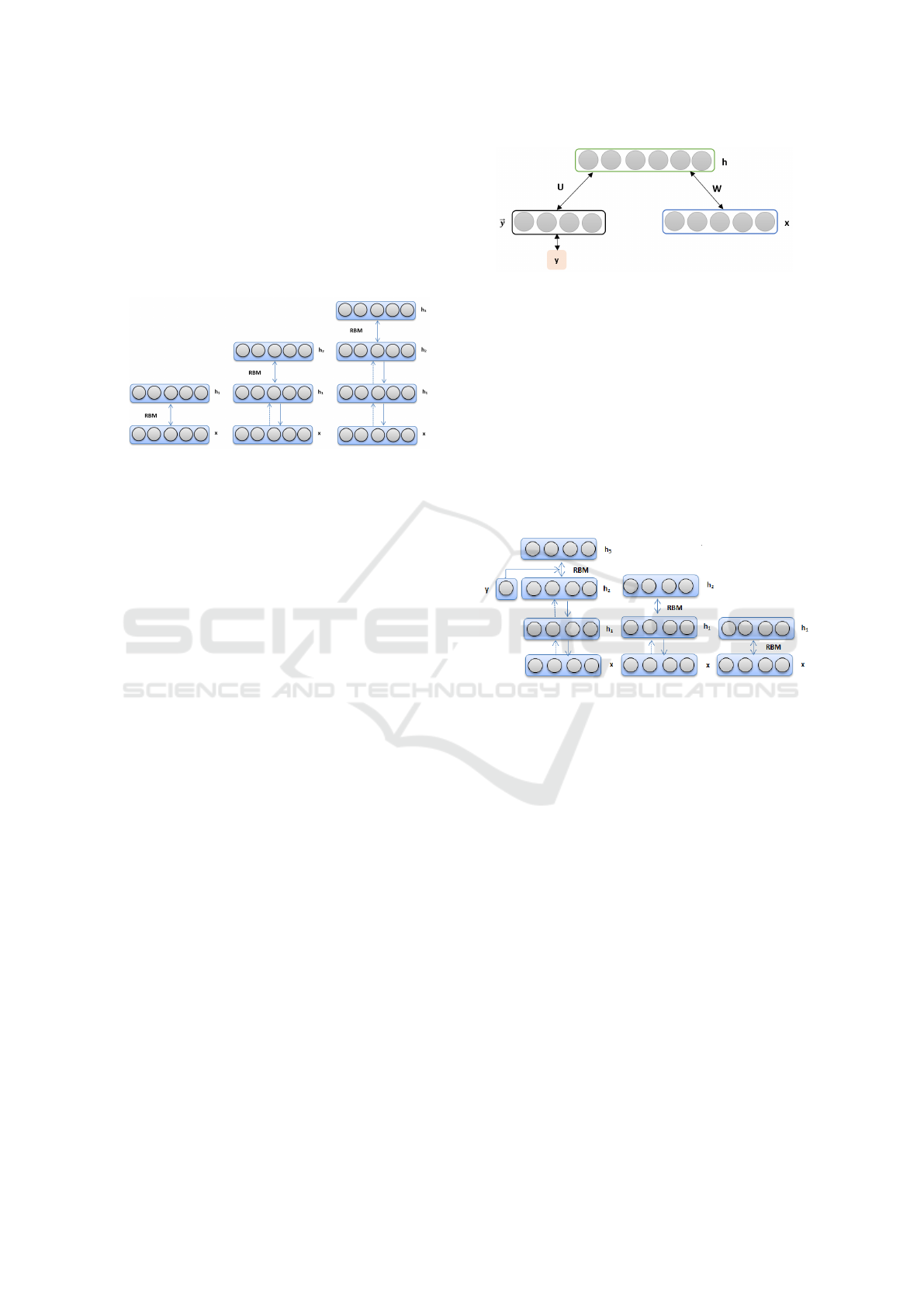
ing weights of all layers together. Figure 5 illustrates
a generative DBN architecture with one visible layer
and three hidden layers.
Figure 5: Generative DBN architecture (GDBN).
5.2 Discriminative Deep Belief Network
(DDBN)
5.2.1 Discriminative Restricted Boltzmann
Machines (DRBMs)
RBMs are used as generative models for various ap-
plications. They use a layer of hidden variables for
modeling the scattering over visible variables. Those
models are typically trained only for modeling the in-
puts of a classification task. They are also capable of
modeling the joint distribution of the inputs and their
associated target classes similar to the last layer of a
DDBN (see 7). We are interested in such joint models
for a classification application.
In this work (Larochelle and Bengio, 2008), the
authors propose a Discriminative Restricted Boltz-
mann Machines which aim to train a density model
by means of a particular RBM consisting of two sets
of visible elements. RBM acts as a parametric model
of joint distribution among a layer of hidden variables
h = (h
1
,..., h
n
) and the visible variables of the inputs
x = (x
1
,..., x
d
) and the target y, that is defined as:
p(y, x,h) ∝ e
−E(y,x,h)
(3)
where
E(y,x, h) = −h
0
W x − b
0
x − c
0
h − d
0
~y − h
0
U~y (4)
with Θ = (W, b,c, d,U) is the set of parameters and
~y = (1
y=i
)
c
i=1
for C classes.
5.2.2 DDBN Architecture
DDBN architectures have been proposed for different
applications (Zhou et al., 2010) (Liu et al., 2011). In
Figure 6: Discriminative RBM model (DRBM). RBM mod-
eling the joint distribution of inputs x and target class y (rep-
resented as one-hot vector by~y ) from (Larochelle and Ben-
gio, 2008). Hidden units are denoted by h.
our work, we use a learning algorithm; discriminative
deep belief network (DDBN) based on discriminative
restricted Boltzmann machine (DRBM) as defined in
(Keyvanrad and Homayounpour, 2014).
DBN aims at letting every RBM model in the
structure to obtain a diverse representation of data. In
other words, after RBM is trained, the activity values
from the hidden units act as the training data for a
higher-level RBM learning.
Figure 7: Discriminative DBN architecture (DDBN). The
last RBM models the joint distribution of inputs x and target
class y. Hidden units are denoted by h.
In DDBN, we need to use a DRBM in the last
layer as a classifier for obtaining labels from the in-
put data. The input layer has a N number of units
which is equivalent to the quantity of sample data x.
The label layer has C representing y as the number of
classes. DDBN trains a joint density model through
discriminative RBM and then each conceivable label
is tested with a test vector. The label which contains
the least energy is selected as the best corresponding
class. Afterward, we use the back-propagation tech-
nique through the entire classifier for fine-tuning the
weights for optimal classification.
5.3 Training in GRBM/DRBM
5.3.1 Contrastive Divergence (CD)
CD is the most popular gradient approximation algo-
rithm. CD initializes the Markov chain with a training
data then the binary hidden units are computed. Once
Generative vs. Discriminative Deep Belief Netwok for 3D Object Categorization
103

the method defines binary hidden unit states then the
visible values are recalculated. Lastly, the probabil-
ity of hidden unit instigations is calculated by means
of hidden and visible unit’s values (Carreira-Perpinan
and Hinton, 2005) .
5.3.2 Persistent Contrastive Divergence (PCD)
As the CD sampling has a few drawbacks and is not
precise, PCD method is proposed so that only the last
chain state is used in the preceding update step (Tiele-
man, 2008).
5.3.3 Free Energy in Persistent Contrastive
Divergence (FEPCD)
Numerous insistent chains can be utilized in paral-
lel during PCD sampling and can mention the present
state as fantasy points in each of these chains. How-
ever, there is a blind chain selection and it’s not nec-
essary that the best one is always selected. Recently,
(Keyvanrad and Homayounpour, 2014) proposed a
new sampling method that defines a standard for the
goodness of chain. This method employs free energy
as a measure to acquire best samples from the gen-
erative model that are able to precisely calculate the
gradient of log probability from training data.
6 EXPERIMENTAL RESULTS
In this section, we tested our categorization approach
on Washington RGBD dataset. The training and test-
ing sets contain 14800 point clouds that are computed
using a Xeon(R) 3.50 GHz CPU 32 GB RAM and
K2000 Nvidia card on Ubuntu 14.04. Figure 2 shows
the examples of 3D point clouds from our training set.
Table 1: GDBN/DDBN characteristics that are used in our
experiment.
Characteristics Value
Hidden layers 3
Hidden layer units 300-300-1500
Learn rates 0.3
Epochs 200
Input layer units size of VFH descriptor (308)
We use a GDBN/DDBN with one visible layer
that contains the VFH descriptors of all training sets,
as well as three hidden layers in order to define a
308-300-300-1500 GDBN/DDBN structures. Then,
we train the weights of each layer separately with the
fixed number of epochs equal to 200 (see Table 1).
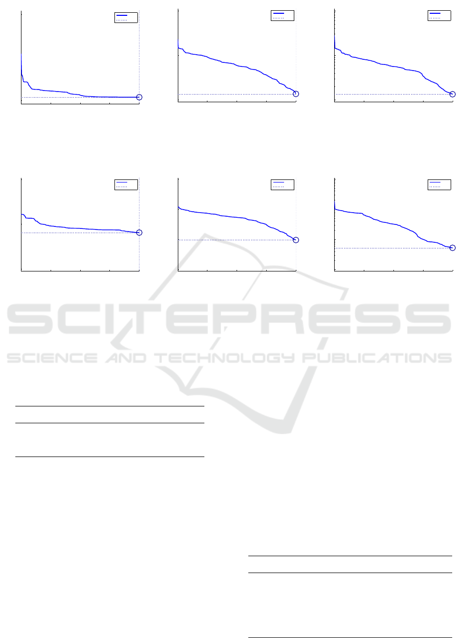
6.1 Evaluation of Generative Model:
GDBN
GDBN aims at allowing each RBM model in the se-
quence to receive a different representation of the
data. In other words, after RBM is trained, the activ-
ity values of its hidden units are used as the training
data for learning a higher-level RBM. As a compar-
ison, we evaluate the training process of GDBN us-
ing CD, PCD or FEPCD training methods. Table 2
shows that the classification error decreases with the
FEPCD training method. We can also remark that
FEPCD training method presents the best accuracy
value. The best training performance indicates the it-
erations at which the validation performance reaches
a minimum mean squared normalized error which is
defined as follows:
MSE =
1
n
n
∑
i=1
(
ˆ
Y
i
−Y
i
)
2
(5)
With:
ˆ
Y
i
is a vector of n predictions, and Y
i
is the vec-
tor of observed values. As shown in Figure 8, the best
performance is obtained with FEPCD training.
Table 2: Classification error and accuracy on Washington
RGBD dataset for 308-300-300-1500 GDBN structure us-
ing different training methods: CD, PCD and FEPCD.
Error Acc.
GDBN-CD 0.6549 34.51%
GDBN-PCD 0.0250 97.5%
GDBN-FEPCD 0.0206 97.9%
6.2 Evaluation of Discriminative Model:
DDBN
The approach trains RBMs one after another and uses
their training data resulting for training stage in the
next RBM using CD, PCD or FEPCD training meth-
ods. The last layer trains a joint density model with
a discriminative RBM. We use the back-propagation
technique through the whole classifier to fine-tune
the weights in order to optimize the classification re-
sult. Table 3 illustrates the classification error be-
fore and after using back-propagation technique. We
notice that the error decreases after using the back-
propagation technique especially with FEPCD train-
ing. Figure 9 shows the best training performance that
indicates the iterations at which the validation perfor-
mance reached a minimum mean squared normalized
error performance criterion. The best performance is
obtained with FEPCD training.
VISAPP 2017 - International Conference on Computer Vision Theory and Applications
104

0 50 100 150 200
10
−1
10
0
Best Training Performance is 0.10789 at epoch 200
Mean Squared Error (mse)
200 Epochs
Train
Best
(CD)
0 50 100 150 200
10
−2
10
−1
10
0
Best Training Performance is 0.013614 at epoch 200
Mean Squared Error (mse)
200 Epochs
Train
Best
(PCD)
0 50 100 150 200
10
−2
10
−1
10
0
Best Training Performance is 0.013379 at epoch 200
Mean Squared Error (mse)
200 Epochs
Train
Best
(FEPCD)
Figure 8: Best training performance on Washington RGBD dataset of 308-300-300-1500 GDBN structure. The minimum
mean squared normalized error 0.013379 is reached at epoch 200 with FEPCD.
0 50 100 150 200
10
−2
10
−1
10
0
Best Training Performance is 0.065007 at epoch 200
Mean Squared Error (mse)
200 Epochs
Train
Best
(CD)
0 50 100 150 200
10
−3
10
−2
10
−1
10
0
Best Training Performance is 0.0095101 at epoch 200
Mean Squared Error (mse)
200 Epochs
Train
Best
(PCD)
0 50 100 150 200
10
−3
10
−2
10
−1
10
0
Best Training Performance is 0.0052535 at epoch 200
Mean Squared Error (mse)
200 Epochs
Train
Best
(FEPCD)
Figure 9: Best training performance on Washington RGBD dataset of 308-300-300-1500 DDBN structure. The minimum
mean squared normalized error 0.0052535 is reached at epoch 200 with FEPCD.
Table 3: Classification errors and accuracy on Washington
RGBD dataset for 308-300-300-1500 DDBN structure us-
ing different training methods: CD, PCD and FEPCD. After
training each RBM, DDBN is fine-tuned in 200 epochs us-
ing the back-propagation method.
Before After Acc.
DDBN-CD 0.3810 0.3155 68.45%
DDBN-PCD 0.4491 0.0201 97.98%
DDBN-FEPCD 0.4053 0.0111 98.89%
6.3 Comparison to Other Methods
In this subsection, we compare our approach to re-
lated state-of-the-art approaches. Table 4 shows the
main accuracy values and compares our 3D recogni-
tion pipeline to the published results (Lai et al., 2011a;
Bo et al., 2011; Schwarz et al., 2015). Lai et al. (Lai
et al., 2011a) extract a set of features that captures the
shape of the object view using spin images, and an-
other set which captures the visual appearance using
SIFT descriptors. These features are extracted sepa-
rately from both depth and RGB images. In contrast,
we extract the geometric features from a single point
cloud using only the VFH descriptor. A recent work
by Schwarz et al. (Schwarz et al., 2015) uses both col-
orizing depth and RGB images that are processed in-
dependently by a convolutional neural network. CNN
features are then learned using SVM classifier in or-
der to successively determine the category, instance,
and pose. In our approach, we use VFH features for
training GDBN/DDBN with three hidden layers that
model a deep network architecture. The results show
also that our recognition pipeline with DDBN arch-
tecture and FEPCD training works perfectly with the
accuracy rate of 98.89% and outperforms all methods
that are mentioned in the state-of-the-art.
Table 4: The accuracy rates on Washington RGBD dataset
for 308-300-300-1500 DDBN structure using CD,PCD and
FEPCD training methods that are compared with the state-
of-the-art methods.
Methods Accuracy rates
CNN (Schwarz et al., 2015) 89.4%
RGBD dataset (Lai et al., 2011a) 64.7%
Depth Kernel (Bo et al., 2011) 78.8%
DDBN-CD 68.45%
DDBN-PCD 97.98%
DDBN-FEPCD 98.89%
Generative vs. Discriminative Deep Belief Netwok for 3D Object Categorization
105

In general, the use of PCD training is better than
CD training, and FEPCD outperforms PCD training.
This result is pertinent, since FEPCD uses free en-
ergy as a criterion for the goodness of a chain in or-
der to obtain elite samples from the generative model
that can more accurately compute the gradient of
the log probability of training data. FEPCD outper-
forms PCD and CD in terms of accuracy, although
its computational complexity is high and takes rela-
tively longer time in training as compared to the two
methods. Our next goal will be to optimize the per-
formance of FEPCD in order to reduce the computa-
tional complexity.
7 CONCLUSIONS
In this work, we focused on 3D object categorization
using geometric features extracted from Viewpoint
Feature Histogram (VFH) descriptor and learned with
both Generative and Discriminative Deep Belief Net-
work (GDBN/DDBN) architectures. GDBN is the
probabilistic model with many Restricted Boltzmann
Machines (RBMs) which are trained sequentially. On
the other hand, DDBN is constructed from the Dis-
criminative Restricted Boltzmann Machine (DRBM)
which is based on RBM and the joint distribution
model. The experimental results using DDBN are en-
couraging, especially that our approach is able to rec-
ognize 3D objects under different views. In a future
work, we will attempt to embed our algorithm in our
robot TurtleBot2 in order to grasp the real-world ob-
jects. Moreover, we will utilize a hybrid deep archi-
tecture that combines the advantage of generative and
discriminative models.
REFERENCES
Aldoma, A., Tombari, F., Rusu, R., and Vincze, M. (2012).
OUR-CVFH–Oriented, Unique and Repeatable Clus-
tered Viewpoint Feature Histogram for Object Recog-
nition and 6DOF Pose Estimation. Springer.
Aldoma, A., Vincze, M., Blodow, N., Gossow, D., Gedikli,
S., Rusu, R., and Bradski, G. (2011). Cad-model
recognition and 6dof pose estimation using 3d cues. In
Computer Vision Workshops (ICCV Workshops), 2011
IEEE International Conference on, pages 585–592.
IEEE.
Alexandre, L. A. (2016). 3d object recognition using con-
volutional neural networks with transfer learning be-
tween input channels. In Intelligent Autonomous Sys-
tems 13, pages 889–898. Springer.
Azevedo, F. A., Carvalho, L. R., Grinberg, L. T., Farfel,
J. M., Ferretti, R. E., Leite, R. E., Lent, R., Herculano-
Houzel, S., et al. (2009). Equal numbers of neuronal
and nonneuronal cells make the human brain an iso-
metrically scaled-up primate brain. Journal of Com-
parative Neurology, 513(5):532–541.
Basu, J. K., Bhattacharyya, D., and Kim, T.-h. (2010). Use
of artificial neural network in pattern recognition. In-
ternational Journal of Software Engineering and Its
Applications, 4(2).
Bo, L., Ren, X., and Fox, D. (2011). Depth kernel descrip-
tors for object recognition. In Intelligent Robots and
Systems (IROS), 2011 IEEE/RSJ International Con-
ference on, pages 821–826. IEEE.
Carreira-Perpinan, M. A. and Hinton, G. E. (2005). On
contrastive divergence learning. In Proceedings of the
tenth international workshop on artificial intelligence
and statistics, pages 33–40. Citeseer.
Deng, L. (2014). A tutorial survey of architectures, algo-
rithms, and applications for deep learning. APSIPA
Transactions on Signal and Information Processing,
3:e2.
Hinton, G. E., Osindero, S., and Teh, Y.-W. (2006a). A
fast learning algorithm for deep belief nets. Neural
computation, 18(7):1527–1554.
Hinton, G. E., Osindero, S., and Teh, Y.-W. (2006b). A
fast learning algorithm for deep belief nets. Neural
computation, 18(7):1527–1554.
Janoch, A., Karayev, S., Jia, Y., Barron, J. T., Fritz, M.,
Saenko, K., and Darrell, T. (2013). A category-level
3d object dataset: Putting the kinect to work. In Con-
sumer Depth Cameras for Computer Vision, pages
141–165. Springer.
Keyvanrad, M. A. and Homayounpour, M. M. (2014).
Deep belief network training improvement using elite
samples minimizing free energy. arXiv preprint
arXiv:1411.4046.
Lai, K., Bo, L., Ren, X., and Fox, D. (2011a). A large-
scale hierarchical multi-view rgb-d object dataset. In
Robotics and Automation (ICRA), 2011 IEEE Interna-
tional Conference on, pages 1817–1824. IEEE.
Lai, K., Bo, L., Ren, X., and Fox, D. (2011b). A large-
scale hierarchical multi-view rgb-d object dataset. In
Robotics and Automation (ICRA), 2011 IEEE Interna-
tional Conference on, pages 1817–1824. IEEE.
Larochelle, H. and Bengio, Y. (2008). Classification us-
ing discriminative restricted boltzmann machines. In
Proceedings of the 25th international conference on
Machine learning, pages 536–543. ACM.
LeCun, Y., Huang, F. J., and Bottou, L. (2004). Learning
methods for generic object recognition with invari-
ance to pose and lighting. In Computer Vision and
Pattern Recognition, 2004. CVPR 2004. Proceedings
of the 2004 IEEE Computer Society Conference on,
volume 2, pages II–97. IEEE.
Liu, Y., Zhou, S., and Chen, Q. (2011). Discriminative deep
belief networks for visual data classification. Pattern
Recognition, 44(10):2287–2296.
Madry, M., Ek, C. H., Detry, R., Hang, K., and Kragic, D.
(2012). Improving generalization for 3d object cate-
gorization with global structure histograms. In Intelli-
gent Robots and Systems (IROS), 2012 IEEE/RSJ In-
ternational Conference on, pages 1379–1386. IEEE.
VISAPP 2017 - International Conference on Computer Vision Theory and Applications
106

McCann, S. and Lowe, D. G. (2012). Local naive bayes
nearest neighbor for image classification. In Computer
Vision and Pattern Recognition (CVPR), 2012 IEEE
Conference on, pages 3650–3656. IEEE.
Nair, V. and Hinton, G. E. (2009). 3d object recognition
with deep belief nets. In Advances in Neural Informa-
tion Processing Systems, pages 1339–1347.
Ouadiay, F. Z., Zrira, N., Bouyakhf, E. H., and Himmi,
M. M. (2016). 3d object categorization and recogni-
tion based on deep belief networks and point clouds.
In Proceedings of the 13th International Conference
on Informatics in Control, Automation and Robotics,
pages 311–318.
Rumelbart, D. and McClelland, J. (1986). Parallel dis-
tributed processing: Explorations in the microstuc-
tures of cognition.
Rusu, R., Blodow, N., Marton, Z., and Beetz, M. Aligning
point cloud views using persistent feature histograms.
In Intelligent Robots and Systems, 2008. IROS 2008.
IEEE/RSJ International Conference on, pages 3384–
3391.
Rusu, R. and Cousins, S. (2011). 3D is here: Point Cloud
Library (PCL). In IEEE International Conference on
Robotics and Automation (ICRA), Shanghai, China.
Rusu, R. B., Blodow, N., and Beetz, M. (2009). Fast
point feature histograms (fpfh) for 3d registration. In
Robotics and Automation, 2009. ICRA’09. IEEE In-
ternational Conference on, pages 3212–3217. IEEE.
Rusu, R. B., Bradski, G., Thibaux, R., and Hsu, J. (2010).
Fast 3d recognition and pose using the viewpoint fea-
ture histogram. In Intelligent Robots and Systems
(IROS), 2010 IEEE/RSJ International Conference on,
pages 2155–2162. IEEE.
Schwarz, M., Schulz, H., and Behnke, S. (2015). Rgb-
d object recognition and pose estimation based on
pre-trained convolutional neural network features. In
Robotics and Automation (ICRA), 2015 IEEE Interna-
tional Conference on, pages 1329–1335. IEEE.
Serre, T., Kreiman, G., Kouh, M., Cadieu, C., Knoblich, U.,
and Poggio, T. (2007). A quantitative theory of imme-
diate visual recognition. Progress in brain research,
165:33–56.
Smolensky, P. (1986). Information processing in dynamical
systems: Foundations of harmony theory.
Socher, R., Huval, B., Bath, B., Manning, C. D., and Ng,
A. Y. (2012). Convolutional-recursive deep learning
for 3d object classification. In Advances in Neural
Information Processing Systems, pages 665–673.
Tieleman, T. (2008). Training restricted boltzmann ma-
chines using approximations to the likelihood gradi-
ent. In Proceedings of the 25th international confer-
ence on Machine learning, pages 1064–1071. ACM.
Toldo, R., Castellani, U., and Fusiello, A. (2009). A bag of
words approach for 3d object categorization. In Com-
puter Vision/Computer Graphics CollaborationTech-
niques, pages 116–127. Springer.
Tombari, F., Salti, S., and D. Stefano, L. (2010). Unique
signatures of histograms for local surface descrip-
tion. In Computer Vision–ECCV 2010, pages 356–
369. Springer.
Tombari, F., Salti, S., and Stefano, L. (2011). A com-
bined texture-shape descriptor for enhanced 3d fea-
ture matching. In Image Processing (ICIP), 2011 18th
IEEE International Conference on, pages 809–812.
IEEE.
Torralba, A., Murphy, K. P., Freeman, W. T., and Ru-
bin, M. A. (2003). Context-based vision system for
place and object recognition. In Computer Vision,
2003. Proceedings. Ninth IEEE International Confer-
ence on, pages 273–280. IEEE.
Wohlkinger, W. and Vincze, M. (2011). Ensemble of shape
functions for 3d object classification. In Robotics and
Biomimetics (ROBIO), 2011 IEEE International Con-
ference on, pages 2987–2992. IEEE.
Zhang, H., Berg, A. C., Maire, M., and Malik, J. (2006).
Svm-knn: Discriminative nearest neighbor classifica-
tion for visual category recognition. In 2006 IEEE
Computer Society Conference on Computer Vision
and Pattern Recognition (CVPR’06), volume 2, pages
2126–2136. IEEE.
Zhou, S., Chen, Q., and Wang, X. (2010). Discriminative
deep belief networks for image classification. In 2010
IEEE International Conference on Image Processing,
pages 1561–1564. IEEE.
Generative vs. Discriminative Deep Belief Netwok for 3D Object Categorization
107