Optimized 4D DPM for Pose Estimation on RGBD Channels using
Polisphere Models
Enrique Martinez
1
, Oliver Nina
2
, Antonio J. Sanchez
1
and Carlos Ricolfe
1
1
Instituto AI2, Universitat Politecnica de Valencia, C/ Vera s/n, Valencia, Spain
2
CRCV, University of Central Florida, Orlando, U.S.A.
Keywords:
Human Pose Estimation, DPM, RGBD Images, Inverse Kinematics.
Abstract:
The Deformable Parts Model (DPM) is a standard method to perform human pose estimation on RGB images,
3 channels. Although there has been much work to improve such method, little work has been done on
utilizing DPM on other types of imagery such as RGBD data. In this paper, we describe a formulation of
the DPM model that makes use of depth information channels in order to improve joint detection and pose
estimation using 4 channels. In order to offset the time complexity and overhead added to the model due to
extra channels to process, we propose an optimization for the proposed algorithm based on solving direct and
inverse kinematic equations, that form we can reduce the interested points reducing, at the same time, the time
complexity. Our results show a significant improvement on pose estimation over the standard DPM model on
our own RGBD dataset and on the public CAD60 dataset.
1 INTRODUCTION
Human pose estimation is a problem that in recent
years has gained much attention. Some of the most
well known methods for human pose estimation are
based on the Deformable Parts Model (Felzenszwalb
et al., 2008; Felzenszwalb et al., 2010; Yang and Ra-
manan, 2013).
Although, there has been a lot of work on recent
years on attempting to improve the DPM model, little
work has been done on utilizing the DPM model on
3D vision channels such as RGBD.
In this work, we propose a new formulation for
the DPM model that takes advantage of depth infor-
mation on RGBD images in order to improve the de-
tection of parts of the model as well as the overall
human pose estimation.
We also reduce the computational cost of train-
ing and testing a DPM model with increased num-
ber of channels by a novel approach solving kine-
matic equations. More specifically, our method treats
each part of the body as a semi rigid object and
use Denavit-Hartemberg (DH) (Waldron Prof and
Schmiedeler Prof, 2008; Khalil and Dombre, 2004)
to solve direct and inverse kinematics equations in or-
der to lower the time complexity of our algorithm.
1.1 Background
Felzenszwalb (Felzenszwalb and Huttenlocher, 2005)
presented a computationally efficient framework for
part-based modeling and recognition using RGB
channels. Saffari (Saffari et al., 2009) introduced an
on-line random forest algorithm also for pose estima-
tion prediction.
One of the most popular methods for pose estima-
tion prediction was published by Ramanan (Felzen-
szwalb et al., 2008; Felzenszwalb et al., 2010; Yang
and Ramanan, 2013). Ramanan’s original model uses
a human detection system based on mixtures of mul-
tiscale Deformable Parts Model (DPM) using RGB
images.
There has been other methods attempting to solve
pose estimation such as Wang (Wang et al., 2012)
who considers the problem of parsing human poses
and recognizing their actions with part-based models
introducing hierarchical poselets.
Shotton (Shotton et al., 2013) proposed a method
to quickly and accurately predict 3D positions of body
joints from a single depth image. Song (Song and
Xiao, 2014) proposed to use depth maps for object
detection and design a 3D detector to overcome major
difficulties of recognition.
In this paper we introduce a novel DPM model
base on Ramanan’s original method with the goal
Martinez E., Nina O., SÃ ˛anchez A. and Ricolfe C.
Optimized 4D DPM for Pose Estimation on RGBD Channels using Polisphere Models.
DOI: 10.5220/0006133702810288
In Proceedings of the 12th International Joint Conference on Computer Vision, Imaging and Computer Graphics Theory and Applications (VISIGRAPP 2017), pages 281-288
ISBN: 978-989-758-226-4
Copyright
c
 2017 by SCITEPRESS – Science and Technology Publications, Lda. All rights reserved
281

to take advantage of additional channels such as the
depth channel in RGBD data. The intuition behind
our approach is that by using depth channels, we
leverage additional 3D position information about the
objects and the scene in the image. Thus, we obtain
a more robust method against image artifacts such as
color, illumination, among others.
Furthermore, we propose an optimization for our
4D DPM model that reduces the number of parts to
be trained. Thus, we are able to successfully reduce
26 parts from the original DPM model to only 10.
This optimization reduces the computational cost of
the model while still preserving high degree of accu-
racy. In the next sections we describe our method in
detail and present our results.
2 PROPOSED METHOD
In this section we describe the propoused method in
three steps. First we explain our formulation of the
Deformable Parts Model to accommodate for addi-
tional channels such as the depth channel. Then we
talk about the pre-processing step for the Depth chan-
nel in which we make a foreground segmentation to
improve the accuracy of our algorithm. Finally, we
explain the optimization of the computation complex-
ity of our model.
2.1 4D DPM Model
We extend the original DPM model by Ramanan
(Felzenszwalb et al., 2010; Yang and Ramanan, 2013)
which is used for articulated human detection and hu-
man pose estimation by creating a new formulation
that extends to alternative channels.
More formally, let us define the score function for
a configuration of parts as a sum of local and pairwise
scores (co-occurrence model):
S (t) =
∑
i∈V
b
t
i
i
+
∑
i j∈E
b
t
i
,t
j
i j
(1)
where i ∈
{
1,...K
}
and K is the number of parts of
the model. t
i
∈
{
1,...T
}
and t
i
is the type of part i. b
t
i
i
is a parameter that favors particular type assignments
for part i, while the pairwise parameter b
t
i
,t
j
i j
favors
particular co-occurrences of part types.
Let us also define G = (V,E) for a K-node rela-
tional graph whose edges specify which pairs of parts
are constrained to have consistent relations.
Hence the score function associated with a con-
figuration of part types and positions for all RGBD
channels is defined as:
S (I, p,t) = S (t)+
∑
i∈V
"
ω
t
i
i
rgb
· φ

I
rgb
, p
i

ω
t
i
i
depth
· φ

I
depth
, p
i

#
+ (2)
+
∑
i j∈E
"
ω
t
i
,t
j
i j
rgb
· υ(p
i
− p
j
)
rgb
ω
t
i
,t
j
i j
depth
· υ(p
i
− p
j
)
depth
#
where φ

I
rgb
, p
i

and φ

I
depth
, p
i

are feature
vectors from RGB (I
rgb
) and Depth (I
depth
) images
respectively and extracted from pixel location p
i
.
We define υ(p
i
− p
j
)
rgb
=

dx dx
2
dy dy
2

rgb
,
where dx = x
i
− x
j
and dy = y
i
− y
j
, is the relative
location of part i with respect to j on image I
rgb
, and
in a similar way for I
depth
.
The second term in equation 2 is an appearance
model that computes the local score of placing a tem-
plate ω
t
i
i
rgb
or ω
t
i
i
depth
for part i, tuned for type t
i
at
location p
i
.
The third term in equation 2 can be interpreted
as a switching spring model that controls the relative
placement of part i and j by switching between a col-
lection of springs. Each spring is tailored for a partic-
ular pair of types (t
i
,t
j
), and is parameterized by its
rest location and rigidity, which are encoded by ω
t
i
i
rgb
or ω
t
i
i
depth
depending on which image is used.
The goal is to maximize S (x, p,t) from the above
formulation over p and t. When the relational graph
G = (V,E) is a tree, this can be done efficiently
with dynamic programing in the following way. Let
kids(i) be the set of children of part i in G. We com-
pute the message part i that passes to its parent j in
this way:
score
i
(t
i
, p
i
) = b
t
i
i
+
"
ω
i
t
i
rgb
· φ

I
rgb
, p
i

ω
i
t
i
depth
· φ

I
depth
, p
i

#
+ (3)
+
∑
k∈kids(i)
m
k
(t
i
, p
i
)
m
i
(t
j
, p
j
) = max
t
i
b
t
i
,t
j
i j
+ max
p
i
score(t
i
, p
i
) + (4)
+
"
ω
t
i
,t
j
i j
rgb
· υ(p
i
− p
j
)
rgb
ω
t
i
,t
j
i j
depth
· υ(p
i
− p
j
)
depth
#
Equation 3 computes the local score of part i, at all
pixel locations p
i
and for all possible types t
i
, by col-
lecting messages from the children of i. Equation 4
computes every location and type of its child part i.
Once messages are passed to the root part (i = 1),
score
1
(c
1
, p
1
) represents the best scoring configura-
tion for each root position and type.
Figure 1 shows our 4D DPM model learned with
only 10 parts, trained on our dataset. We show the
VISAPP 2017 - International Conference on Computer Vision Theory and Applications
282

local templates in Figure 1 part (a), and the tree struc-
ture in Figure 1 part (b), placing parts at their best-
scoring location relative to their parent.
Though we visualize 4 trees generated by select-
ing one of the four types of each part, and placing it at
its maximum-scoring position, there exists an expo-
nential number of possible combinations, obtained by
composing different part types together. Notice that
the standard DPM model consists of 14 or 26 parts
which are used on RGB images only. In our case we
only need 10 parts to train and test our model. The
reason for this is to reduce the computational com-
plexity of the model which we explain in more detail
in section 2.3.
Figure 1: Our Learned Model: 10 parts using our dataset.
(a): the local templates. (b): the tree structure.
2.2 Foreground Segmentation
Although D channels in RGBD data provide impor-
tant information about location of the target object,
it is still necessary to make a foreground segmenta-
tion from the target object. By making the foreground
segmentation, we accent the image contrast between
foreground and background as well as remove any
noise that could negatively affect our model.
In order to automatically make a foreground seg-
mentation from depth channels, we use a Maxi-
mally Stable Extremal Regions (MSER) based ap-
proach (Matas et al., 2004). MSER regions are re-
gions that are most stable through a range of all possi-
ble threshold values applied to them. More formally:
Given a seed pixel x, and a parameter ∆ which rep-
resents the intensity variation in the scale of x, we de-
fine the stability property S of a region R as:
S =
|∆R − R|
|R|
(5)
where the unary operator || represents the area of the
region input. Hence, MSER regions are those with
higher S values.
Given a Depth channel image, we use equation 5
to obtain the most stable regions from the channel.
We then remove those MSRE regions that hold the
following property
|R| > T (6)
where T is a certain threshold for the area of the re-
gion. We can see in Figure 2 the results from our
segmentation method.
Figure 2: (a) Original Depth, (b) Depth after applying
MSER; (c) Conversion of Depth pixel position to RGB pixel
position; (d) Original RGB; (e) Combining image (c) and
(d).
2.3 Model Optimization
The additional Depth channel included in proposed
formulation of DPM adds extra computational cost
that makes training and testing cumbersome.
In this section we explain an optimization tech-
nique that makes use of inverse kinematic equations in
order to infer other parts by training with fewer ones.
We will first describe the system and calibration pro-
cess we use in order to use the propoused optimization
step.
2.3.1 3D Vision System
The proposed vision system used in our experiments
is the Kinect camera, which consists of two optical
sensors whose interaction allows a three-dimensional
scene analysis.
One of the sensors is a RGB camera which has a
video resolution of 30 fps. The image resolution given
by this camera is 640x480 pixels. The other sensor
is an infrared camera that gathers depth information
from objects found in the scene.
The main purpose of this sensor is the emission of
an infrared signal which is reflected off of objects be-
ing visualized and then recaptured by a monochrome
CMOS sensor. A matrix is then obtained which
provides a depth image of the objects in the scene.
Hence, calibration at this stage is much needed to cor-
relate both camera and world coordinate system.
Optimized 4D DPM for Pose Estimation on RGBD Channels using Polisphere Models
283

2.3.2 3D Vision System Calibration
The intrinsic and extrinsic parameters of the two
Kinect optical sensors are different. Therefore, it is
necessary to calibrate one optical sensor (RGB) with
respect to the other (Depth) in order to correlate the
corresponding pixels in both images. The calibration
system is done in a similar way to (Berti et al., 2012)
or (Viala et al., 2011) and (Viala et al., 2012).
Using RGBD information together with a calibra-
tion system, we can know where a pixel is on an im-
age with respect to the camera, we can also convert
a point in pixel coordinates

x
pixel
,y
pixel

(2D coor-
dinates inside the image) to another point in camera
coordinates (x
camera
,y
camera
,z
camera
) (3D coordinates
of one point in the world with respect to the camera).
Thus, we use the point in camera coordinates to cal-
culate the kinematic equations.
2.4 Model of Human Body using
Polispheres
In order to track the human skeleton, it is necessary to
perform the modeling of the human body. The human
body is modeled as a set of articulated rigid structures
to perform the necessary simplifications and to obtain
a simple model. For each of these articulated rigid
structures the state variables and kinematics are ob-
tained. Kinematics are calculated using DH (Denavit-
Hartemberg).
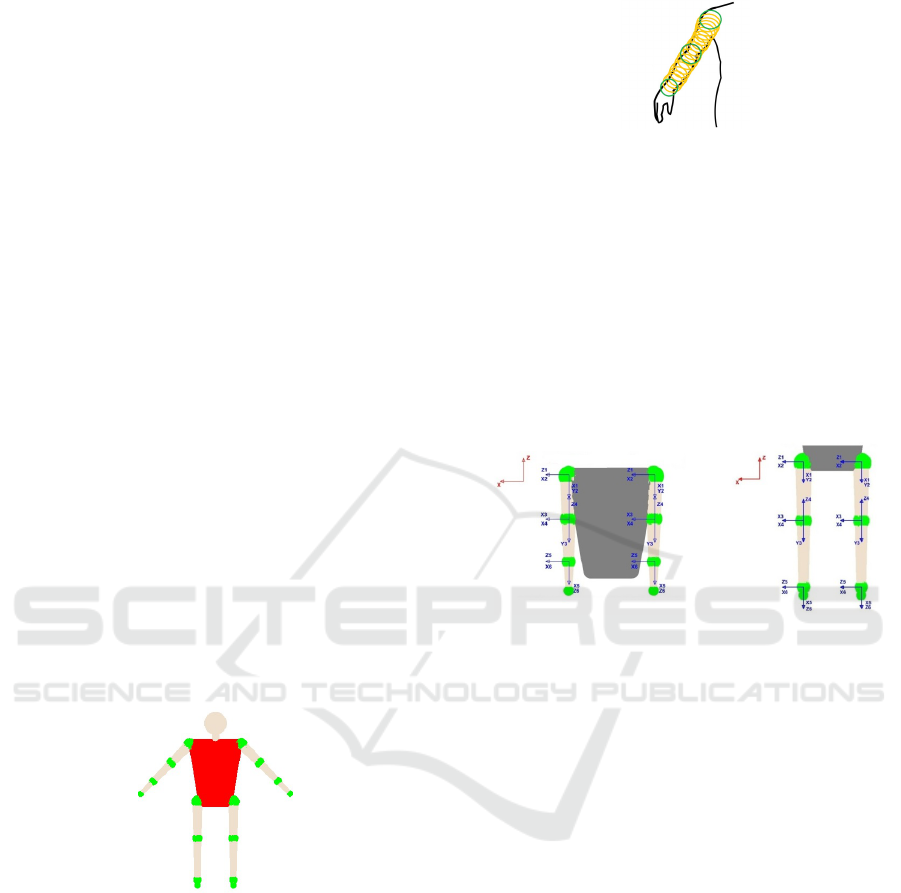
Figure 3: Body human model.
Figure 3 shows the geometrical model used, where
the green spheres indicate the main areas to represent
each of the limbs.
For use polysphere, we have modeled each part of
the body using two points, between these two points
we have one number defined of spheres, the first and
the last one represents our articulations. The body are
modeled using 4 points (hips and shoulders). Figure 4
shows a representation of polisphere model used.
Figure 4: Polisphere representation. Green: sphere cen-
tered on articulated join. Yellow: spheres encompassing the
shaped part of the body.
2.5 State Variable
The human body is designed as if it were a set of artic-
ulated rigid structures performing collision detection.
More concretely, our human body model is composed
of 4 different articulated rigid structures: 1 structure
for each arm and 1 structure for each leg. Also, state
variables for each of these articulated rigid structures
are created.
Figure 5: State Variable. Left: arms, Right: legs.
2.5.1 Denavit Hartemberg (DH)
To control each of these articulated rigid structures to
which human body model has been reduced to, we
use DH (Waldron Prof and Schmiedeler Prof, 2008;
Khalil and Dombre, 2004). We use 6 joints for each
articulated rigid structure, starting with shoulders or
hips and ending with hands or feet respectively.
First, we establish the base coordinate system
(X
0
,Y
0
,Z
0
) at the supporting base with Z
0
axis ly-
ing along the axis of motion of joint 1. We estab-
lish a joint axis and align the Z
i
with the axis of
motion of joint i + 1. We also locate the origin of
the i
th
coordinate at the intersection of the Z
i
and
Z
i−1
or at the intersection of a common normal be-
tween the Z
i
and Z
i−1
. Then, we establish X
i
=
±(Z
i−1
× Z
i
)/
k
Z
i−1
× Z
i
k
or along the common nor-
mal between the Z
i
and Z
i−1
axes when they are par-
allel. We also assign Y
i
to complete the right-handed
coordinate system. Finally, we find the link and joint
parameters: θ
i
, d
i
, a
i
, α
i
. Figure 5 shows our kine-
matic model.
We can use this information to calculate the in-
verse and direct kinematics. For direct kinemat-
ics, given the 6 variable joints (q
1
,q
2
,q
3
,q
4
,q
5
,q
6
),
VISAPP 2017 - International Conference on Computer Vision Theory and Applications
284

we obtain the coordinates of end effector (x,y, z)
with respect the base of the articulated rigid struc-
ture. For inverse kinematics, given the coordinates
of end effector and the orientation in euler parame-
ters, (x,y, z,φ,θ,ψ), we obtain the 6 variable joints,
(q
1
,q
2
,q
3
,q
4
,q
5
,q
6
).
Using the information above, we calculate direct
kinematics using a homogeneous transformation ma-
trix:
i−1
A
i
(q
i
) = (7)



c(θ
i
) −c(α
i
) · s (θ
i
) s(α
i
) · s (θ
i
) a
i
· c (θ
i
)
s(θ
i
) c(α
i
) · c (θ
i
) −s (α
i
) · c (θ
i
) a
i
· s (θ
i
)
0 s(α
i
) c(α
i
) d
i
0 0 0 1



Equation 7 relates a joint with the previous. We
need identify the location of the end effector relative
to the reference, equation 8 show the matrix necessary
to do it:
0
T
6
(q
1
,q
2
,q
3
,q
4
,q
5
,q
6
)=
0
A
1
(q
1
)·
1
A
2
(q
2
)· (8)
·
2
A
3
(q
3
)·
3
A
4
(q
4
)·
4
A
5
(q
5
)·
5
A
6
(q
6
)
To calculate inverse kinematics is necessary use
geometric models for the first three joints because it
can not be done using the inverse transform technique.
We have the coordinates for the final effector (x,y,x)
and after apply geometric models we obtain the first
three joints:
q
1
= arctan

y
x

(9)
q
3
= arctan




±
r
1 − cos
2

x
2
+y
2
+z
2
−a
2
−a
3
2·a
2
·a
3

cos

x
2
+y
2
+z
2
−a
2
−a
3
2·a
2
·a
3





(10)
q
2
= arctan
z
±
p
x
2
+ y
2
!
− (11)
−arctan


a
3
· sin

x
2
+y
2
+z
2
−a
2
−a
3
2·a
2
·a
3

a
2
+ a
3
· cos

x
2
+y
2
+z
2
−a
2
−a
3
2·a
2
·a
3



Now we can use inverse kinematics to calculate
the last three joints. We write
0
R
6
= [n o a] =
0
R
3
·
3
R
6
for the sub matrix rotation of
0
T
6
. We know
0
R
6
because is the orientation of the final effector and
0
R
3
because is defined by
0
R
3
=
0
R
1
·
1
R
2
·
2
R
3
using
(q
1
,q
2
,q
3
). Then we need calculate:
3
R
6
= [r
i j
] =

0
R
3

−1
0
R
6
(12)
Applying
3
R
6
=
3
R
4
·
4
R
5
·
5
R
6
using (q
4
,q
5
,q
6
),
we obtain equation 13.
3
R
6
= (13)


a + b a − b −c(q
4
)s (q
5
)
c − e d + f −s(q
4
)s (q
5
)
c(q
6
)s (q
5
) s(q
6
)s (q
5
) c(q
5
)


W here :
a = c (q
4
)c (q
5
)c (q
6
) b = s (q
4
)s (q
6
)
c = s (q
4
)c (q
5
)c (q
6
) d = s(q
4
)c (q
5
)s (q
6
)
e = c (q
4
)s (q
6
) f = c (q
4
)c (q
6
)
We obtain the last three joints using equation 12
and equation 13:
q
4
= arctan

r
23
r
13

(14)
q
5
= arccos(−r
33
) (15)
q
6
=
π
2
− arctan

r
32
r
31

(16)
In our case, we use inverse kinematics because
we can obtain where the base of our articulated rigid
structure (shoulders or hips) is, and where the fi-
nal effector and the orientation (hands an feet) are,
thus we have these parameters: (x, y,z,φ, θ,ψ) and
using inverse kinematics, we obtain the 6 variable
joints,(q
1
,q
2
,q
3
,q
4
,q
5
,q
6
), and use them to know
where the elbow or knee is located. Algorithm 1
shows the steps of our method.
Algorithm 1: Algorithm used.
1: Data: RGB and Depth image.
2: Result: Human body pose estimation.
3: Initialization.
4: Load model trained.
5: Load frames.
6: for i = 1 : nFrame do
7: Read RGB and Depth.
8: Apply MSER.
9: Convert pixel depth to pixel RGB.
10: Obtain points from DPM.
11: Convert points to 3D coordinates.
12: Apply DH.
13: Visualization.
14: end for
15: Obtain APK and PCK acuracy.
16: Obtain error metrics.
3 RESULTS
For the evaluation of our results, we use a similar
method to (Yang and Ramanan, 2013), where a PCK
and APK metrics are used. In PCK we use test images
Optimized 4D DPM for Pose Estimation on RGBD Channels using Polisphere Models
285

with tightly-cropped bounding box for each person.
Given the bounding box, a pose estimation algorithm
reports back keypoint locations for body joints.
A candidate keypoint is defined to be correct if it
falls within α · max(h,ω) pixels of the ground-truth
keypoint, where h and ω are the height and width of
the bounding box respectively, and α controls the rel-
ative threshold for considering correctness.
For the APK metric, is not necessary the access
to the bounding box. One can combine the two prob-
lems by thinking of body parts as objects to be de-
tected, and evaluate object detection accuracy with a
precision-recall curve (Everingham et al., 2010).
We consider a candidate key point to be correct if
it lies within α · max(h,ω) pixels of the ground-truth.
Thus, we obtain values in the range of 0% and 100%;
Hence the higher the value, the better the accuracy.
The second method consists in directly calculat-
ing the distance between the results and the correct
labeled point. To do this, we use a set of images where
all joints have been labeled. The distance between the
result and the correct location label represents an error
score. For each joint we obtain an error score which
is the mean value calculated from all frames.
3.1 Quantitative Results
3.1.1 Foreground Segmentation Evaluation
For our foreground segmentation evaluation method,
we use in all cases 6 mixtures parts. The size of the
images are 320x240.
The results presented here evaluate the relevance
of using our foreground segmentation method. Ta-
ble 1 shows the results of using foreground segmenta-
tion in either the testing or training phases.
Table 1: APK, PCK and Error Metrics For Foreground Seg-
mentation.
Model B. training B. testing keypoint head shoulder wrist hip ankle mean
1 no no
APK 100 100 89.64 100 100 97.92
PCK 100 100 92.42 100 100 98.48
error 4.22 3.66 7.63 5.96 4.43 5.18
2 no yes
APK 100 100 83.79 100 100 96.75
PCK 100 100 89.39 100 100 97.87
error 4.54 3.61 7.70 3.35 3.77 4.59
3 yes no
APK 100 100 82.40 100 100 96.49
PCK 100 100 87.37 100 100 97.47
error 3.03 4.49 9.65 3.38 3.09 4.72
4 yes yes
APK 100 100 95.63 100 100 99.12
PCK 100 100 96.46 100 100 99.29
error 2.55 4.70 5.62 3.41 2.64 3.78
“B. training” represents the use of foreground seg-
mentation on the training image and “B. testing” rep-
resents the use a foreground segmentation on the test
image.
Table 1 shows that our method with foreground
segmentation, obtains accuracies of around 99%. We
can corroborate these results with our second eval-
uation, where we obtain the distance between two
points. In this case, Table 1 shows our method
achieves an average error of only 3.78 compared
to 5.18, where no foreground segmentation is per-
formed.
3.1.2 Complete Model Evaluation
3.1.3 Our Dataset
Our dataset consists of 7 videos with only one per-
son on the scene moving his arms and legs. In total
we have around 1000 images were people are mov-
ing their arms and legs. All of these images are in
the same scene but with different objects and differ-
ent clothes.
We compare our method which uses 6 mixture
parts and 10 parts, with the original DPM model
which uses 6 mixture parts and 26 parts. We train
both models with the same training samples from our
own dataset.
Table 2: APK, PCK and Error Metrics For Complete
Method.
Model keypoint head shoulder wrist hip ankle mean
DPM
APK 100 100 78.04 100 100 95.60
PCK 100 100 83.33 100 100 96.66
error 4.48 6.29 18.53 3.94 4.25 7.49
Ours
APK 100 100 95.63 100 100 99.12
PCK 100 100 96.46 100 100 99.29
error 2.55 4.70 5.62 3.41 2.64 3.78
We can observe in Table 2 that our method outper-
forms the standard DPM model, specially on the wrist
part with about 3% better accuracy. We can also see
that our method achieves lower error rates in all the
parts compared to the standard DPM.
3.1.4 CAD60 Dataset
The CAD60 dataset contains 60 RGB-D videos, 4
subjects (two male, two female), 5 different environ-
ments (office, bedroom, bathroom and living room)
and 12 activities (rinsing mouth, brushing teeth, wear-
ing contact lens, talking on the phone, drinking wa-
ter, opening pill container, cooking (chopping), cook-
ing (stirring), talking on couch, relaxing on couch,
writing on whiteboard, working on computer). The
dataset also provides ground truth for the joints of the
skeletons that belong to the subjects in the videos.
VISAPP 2017 - International Conference on Computer Vision Theory and Applications
286

The CAD60 dataset has been used succesfully for
activity recognition as in (Ni et al., 2013; Gupta et al.,
2013; Wang et al., 2014; Shan and Akella, 2014;
R. Faria et al., 2014). However, our problem is not
activity recognition but human pose estimation. Nev-
ertheless, because ground truth for the joints are pro-
vided with CAD60, this dataset fulfills our needs well.
Because there are not many publicly available
RGBD datasets that provide ground truth joints of
subjects, we are limited to use CAD60. Also, to our
knowledge, there is no published results on human
pose estimation for this dataset. Because of this and
because there are not many non-commercial and pub-
licly available methods that deal with RGBD data for
pose estimation, we compare our method only to the
original DPM model.
For these experiments, our model is trained using
the samples from CAD60 dataset. We compare our
method to a previously trained DPM model and an-
other DPM model trained solely on CAD60 samples
(DPM-t).
Table 3: APK and PCK metrics on the CAD60 dataset.
Model keypoint head shoulder wrist hip ankle mean
DPM
APK 47.42 66.69 22.95 45.98 47.10 46.02
PCK 62.00 70.50 39.00 60.00 57.50 57.80
error 17.35 14.10 35.89 7.06 19.57 18.79
DPM-t
APK 73.02 73.53 32.26 66.33 42.38 57.50
PCK 78.50 78.50 44.50 70.50 49.50 64.30
error 15.21 12.30 31.02 6.64 16.31 16.29
P. Method
APK 91.23 87.06 51.63 86.21 82.01 79.63
PCK 92.80 90.00 66.00 89.00 90.00 85.56
error 8.81 7.53 19.25 6.05 9.25 10.17
Table 3 shows our method outperforms the stan-
dard DPM model by a large margin of about 20% ac-
curacy. Table 3 also show the errors rates between
correct points and points detected. We can observe
that using our model we have around 10 points less of
error rate than the standard DPM model.
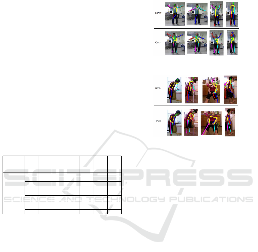
3.2 Qualitative Results
In this section we analyze the qualitative results of
our method. Figure 6 shows different frames where
the original DPM model fails, and where our model
works better on our dataset. Figure 7 shows different
frames where the original DPM model trained with
CAD60 dataset (DPM-t) fails, and where our model
works better on CAD60. The images in the first row in
Figure 6 and Figure 7 show the original DPM model
and the images in the second row represent ours. No-
tice that our model more accurately predicts the pose
of the person in the video.
Figure 8 shows the human model obtained through
Figure 6: Qualitative comparison of DPM and our method
on our proposed dataset.
Figure 7: Qualitative comparison of DPM trained with
CAD60 dataset (DPM-t) and our proposed method on
CAD60.
DH in different frames. Our kinematic model cor-
rectly infers the parts and joints of the human body.
We obtain the solutions in Figure 8 applying DH at
points obtained through our model.
3.3 Time Complexity Analysis
Here we describe the computational cost between the
original DPM model and ours. For our experiments,
we use a windows 7 system with 4 GB RAM. We take
99 frames and we calculate for each frame the origi-
nal DPM model and our model, finally we take the
average time between all frames.
In both cases we use the same size of the image,
320x240. Using the original model we have a compu-
tational cost of 9.21 seconds for each frame whereas
using our model, the computational cost is reduced
to 7.26 seconds even though we are processing more
channels than the original model. This is roughly a
20% gain in performance.
4 CONCLUSIONS
In this paper, we extend a DPM model that takes ad-
vantage of Depth information on RGBD images in
order to improve detection of parts and human pose
estimation.
We also propose a novel foreground segmentation
Optimized 4D DPM for Pose Estimation on RGBD Channels using Polisphere Models
287

Figure 8: Body human model calculated after obtain the
points by our proposed DPM model.
technique ideal for Depth channels of RGBD data that
helps us improve our results further.
Finally, we reduce the computational cost of our
new DPM model by a novel approach solving kine-
matic equations. Our results show significant results
over the standard DPM model in our dataset and in
the publicly available CAD60 dataset.
ACKNOWLEDGEMENTS
This work was partially financed by Plan Nacional
de I+D, Comision Interministerial de Ciencia y Tec-
nologa (FEDER-CICYT) under the project DPI2013-
44227-R.
REFERENCES
Berti, E. M., Salmer
´
on, A. J. S., and Benimeli, F. (2012).
Human–robot interaction and tracking using low cost
3d vision systems. Romanian Journal of Technical
Sciences - Applied Mechanics, 7(2):1–15.
Everingham, M., Van Gool, L., Williams, C. K., Winn, J.,
and Zisserman, A. (2010). The pascal visual object
classes (voc) challenge. International journal of com-
puter vision, 88(2):303–338.
Felzenszwalb, P., McAllester, D., and Ramanan, D. (2008).
A discriminatively trained, multiscale, deformable
part model. In 2013 IEEE Conference on Computer
Vision and Pattern Recognition, pages 1–8. IEEE.
Felzenszwalb, P. F., Girshick, R. B., McAllester, D., and
Ramanan, D. (2010). Object detection with discrim-
inatively trained part-based models. Pattern Analy-
sis and Machine Intelligence, IEEE Transactions on,
32(9):1627–1645.
Felzenszwalb, P. F. and Huttenlocher, D. P. (2005). Pic-
torial structures for object recognition. International
Journal of Computer Vision, 61(1):55–79.
Gupta, R., Chia, A. Y.-S., and Rajan, D. (2013). Human
activities recognition using depth images. In Proceed-
ings of the 21st ACM international conference on Mul-
timedia, pages 283–292. ACM.
Khalil, W. and Dombre, E. (2004). Modeling, identification
and control of robots. Butterworth-Heinemann.
Matas, J., Chum, O., Urban, M., and Pajdla, T. (2004).
Robust wide-baseline stereo from maximally sta-
ble extremal regions. Image and vision computing,
22(10):761–767.
Ni, B., Pei, Y., Moulin, P., and Yan, S. (2013). Multi-
level depth and image fusion for human activity detec-
tion. Cybernetics, IEEE Transactions on, 43(5):1383–
1394.
R. Faria, D., Premebida, C., and Nunes, U. (2014). A
probalistic approach for human everyday activities
recognition using body motion from rgb-d images.
IEEE RO-MAN’14: IEEE International Symposium
on Robot and Human Interactive Communication.
Saffari, A., Leistner, C., Santner, J., Godec, M., and
Bischof, H. (2009). On-line random forests. In
Computer Vision Workshops (ICCV Workshops), 2009
IEEE 12th International Conference on, pages 1393–
1400. IEEE.
Shan, J. and Akella, S. (2014). 3d human action segmenta-
tion and recognition using pose kinetic energy. IEEE
Workshop on Advanced Robotics and its Social Im-
pacts (ARSO).
Shotton, J., Sharp, T., Kipman, A., Fitzgibbon, A., Finoc-
chio, M., Blake, A., Cook, M., and Moore, R. (2013).
Real-time human pose recognition in parts from sin-
gle depth images. Communications of the ACM,
56(1):116–124.
Song, S. and Xiao, J. (2014). Sliding shapes for 3d object
detection in depth images. In Computer Vision–ECCV
2014, pages 634–651. Springer.
Viala, C. R., Salmeron, A. J. S., and Martinez-Berti, E.
(2011). Calibration of a wide angle stereoscopic sys-
tem. OPTICS LETTERS, ISSN 0146-9592, pag 3064-
3067.
Viala, C. R., Salmeron, A. J. S., and Martinez-Berti, E.
(2012). Accurate calibration with highly distorted im-
ages. APPLIED OPTICS, ISSN 0003-6935, pag 89-
101.
Waldron Prof, K. and Schmiedeler Prof, J. (2008). Kine-
matics. Springer Berlin Heidelberg.
Wang, J., Liu, Z., and Wu, Y. (2014). Learning actionlet
ensemble for 3d human action recognition. In Human
Action Recognition with Depth Cameras, pages 11–
40. Springer.
Wang, Y., Tran, D., Liao, Z., and Forsyth, D. (2012). Dis-
criminative hierarchical part-based models for human
parsing and action recognition. The Journal of Ma-
chine Learning Research, 13(1):3075–3102.
Yang, Y. and Ramanan, D. (2013). Articulated human de-
tection with flexible mixtures of parts. Pattern Anal-
ysis and Machine Intelligence, IEEE Transactions on,
35(12):2878–2890.
VISAPP 2017 - International Conference on Computer Vision Theory and Applications
288