Linear Software Models: Modularity Analysis by the

Laplacian Matrix

Iaakov Exman and Rawi Sakhnini

Software Engineering Dept., The Jerusalem College of Engineering – JCE-Azrieli, Jerusalem, Israel

Keywords: Linear Software Models, Modularity Matrix, Laplacian Matrix, Connected Components, Eigenvectors,

Zero-valued Eigenvalues, Bipartite Graph, Software Redesign, Coupling Resolution, Outliers.

Abstract: We have recently shown that one can obtain the number and sizes of modules of a software system from the

eigenvectors of the Modularity Matrix weighted by an affinity matrix. However such a weighting still

demands a suitable definition of an affinity. This paper obtains the same results by means of a Laplacian

Matrix, directly based upon the Modularity Matrix without the need of weighting. These formalizations are

different alternatives leading to the same outcomes based upon a central idea: modules are connected

components. The important point is that, independently of specific advantages of given techniques, there is

just one single unified algebraic theory of software composition – the Linear Software Models – behind the

different approaches. The specifics of the Laplacian Matrix technique, after its formal enunciation, are

illustrated by calculations made for case studies.

1 INTRODUCTION

Software engineering is an exercise in composition

(Fall, 2016). A software system is composed from

subsystems, which are made of sub-subsystems and

so on for each hierarchy level of the system, down to

indivisible components. The problem to be solved is

which components are needed to satisfy the system

required functionalities. It is widely accepted that

modularity is essential to solve this problem.

Our Linear Software Models approach uses

Modularity Matrices linking component structures to

their functionalities, see (Exman, 2012 and 2013).

The outcome is a set of modules in the respective

hierarchical level of the software system.

Recently we have shown that numbers and sizes

of the referred modules can be precisely obtained

from eigenvectors of the Modularity Matrix suitably

weighted by an affinity matrix (Exman, 2015).

In this paper we show that the same numbers and

sizes of modules are obtained from the eigenvectors

of a Laplacian Matrix, directly derived from the

Modularity Matrix, without the need of weighting.

In this Introduction we review properties of the

Modularity Matrix and the Laplacian Matrix.

1.1 Modularity Matrix Concepts

Modularity is the antithesis of coupling between

software components. Thus, a theory of modular

composition must clearly define coupling. An

intuitive notion of coupling is given in the Design

Patterns GoF book Glossary (Gamma et al., 1995):

coupling is the degree to which software

components depend on each other. In our Linear

Software Models, this is translated to "coupling is

linear dependence" among software components.

To apply the theory, a Modularity Matrix

(Exman, 2014) is constructed for each software

system. The matrix displays relations between the

software system architectural entities: column

structors, and row functionals. Structors generalize

UML classes and functionals generalize methods. A

1-valued matrix element means that the column

structor provides a functional in the respective row.

To avoid couplings, a standard Modularity

Matrix must have all its structors and respectively all

its functionals linearly independent. From linear

algebra it follows that the standard Modularity

Matrix is square. If certain structor sub-sets provide

sub-sets of functionals disjoint to other sub-sets, the

matrix is strictly block-diagonal. These blocks are

the desired independent modules.

100

Exman, I. and Sakhnini, R.

Linear Software Models: Modularity Analysis by the Laplacian Matrix.

DOI: 10.5220/0005985601000108

In Proceedings of the 11th International Joint Conference on Software Technologies (ICSOFT 2016) - Volume 2: ICSOFT-PT, pages 100-108

ISBN: 978-989-758-194-6

In a standard Modularity Matrix modules are

irreducible – cannot be broken into smaller modules.

All the matrix elements outside modules are zero-

valued, the modules are orthogonal thus mutually

linearly independent. One easily shows that

eigenvectors of a suitably weighted Modularity

Matrix precisely reflect module sizes. This spectral

approach (Exman, 2015) is illustrated in Fig. 1.

Figure 1: Schematic Modularity Matrix with a fitting

eigenvector – The square block-diagonal matrix has 4

numbered modules (blue background). The eigenvector at

the right-hand-side of the matrix precisely reflects the size

of module #2 (with hatched background).

1.2 Laplacian Matrix Concepts

A generic Laplacian matrix is defined upon a graph.

For software systems the graph is undirected, and

edges link the referred architectural units – structors

and functionals – where each unit is a vertex in the

graph. Formally the Laplacian

is given by:

LDA

(1)

where D is the Degree Matrix – showing the degree

deg( )iv

of vertex

in its diagonal element iiD –

and

is the Adjacency Matrix – showing for each

,ij

pair of vertices whether they are adjacent in the

graph. Adjacent vertices have a 1-valued

matrix

element and 0-valued otherwise.

Laplacian properties of interest are:



L is symmetric;

 The number of zero-valued eigenvalues of the

Laplacian Matrix is the number of graph

connected components.

1.3 Modules as Connected Components

This paper’s purpose is to show that for:

 strictly block-diagonal Modularity Matrix – the

same results are obtained by means of the

eigenvectors of the Laplacian Matrix;

 case of outliers – a neat procedure is formulated

to highlight residual coupling.

The argument centrepiece is that modules are

connected components. This is true for blocks of the

block-diagonal Modularity Matrix (Exman, 2014),

sub-lattices of a Modularity Lattice (Exman and

Speicher, 2015) or sub-graphs obtaining a Laplacian

Matrix in this paper. One follows the next steps:

Generate a Bipartite Graph – from the

Modularity Matrix;

Obtain the Laplacian Matrix – from the

generated graph;

Software Modules are Connected Components

– seen in the graph and in the corresponding

Laplacian;

Number of Modules – is set by the number of

zero-valued Laplacian eigenvalues;

Sizes of Modules – are given by the non-zero

elements of Laplacian eigenvectors;

Modules Sparsity – may demand module

splitting to assure sparsity below a threshold,

thereby highlighting outlier coupling in need of

redesign.

The above steps will be first intuitively illustrated by

an introductory example. Then, formal proofs will

be provided in a subsequent section.

1.4 Organization of the Paper

The remaining of this paper is organized as follows.

Section 2 mentions related work. Section 3 displays

an introductory example. Section 4 formulates

theoretical considerations. Section 5 presents case-

studies. A discussion concludes the paper.

2 RELATED WORK

2.1 Modularity Analysis

Various techniques are suitable for modularity

analysis. Here is a short sample of approaches.

Baldwin and Clark, in their “Design Rules” book

(Baldwin and Clark, 2000), describe a Design

Structure Matrix (DSM) upon which one adds an

economic design model. DSM has also been applied

to software engineering (Cai and Sullivan, 2006).

Conceptual lattices were introduced in (Wille,

1982) within Formal Concept Analysis (FCA). This

Linear Software Models: Modularity Analysis by the Laplacian Matrix

101

technique has been used for modularization and

software system design, e.g. (Siff and Reps, 1999).

In previous spectral work we have used

eigenvectors of the Modularity Matrix symmetrized

and weighted by an Affinity (Exman, 2015) to

extract software system modules' numbers and sizes.

2.2 Laplacian Matrix Techniques

Spectral techniques based upon the Laplacian Matrix

have been used in various contexts, including

software engineering. A good survey on Laplacian

matrices of graphs is (Merris, 1994).

A tutorial on spectral clustering, with emphasis

on Laplacian techniques is (von Luxburg, 2007). A

more recent review on clustering methodologies for

software engineering, of spectral methods in general

and in particular the Laplacian is (Shtern and

Tzerpos, 2012).

Ng et al. (Ng et al., 2001) deal with spectral

clustering, analysing an algorithm, explicitly

referring to the Laplacian. Shokoufandeh et al.

(Shokoufandeh, 2005) extract a Module Dependency

Graph (MDG) from software source code for

clustering into MDG partitions. Their

Modularization Quality criterion is reformulated as a

Laplacian eigenvalue problem.

3 INTRODUCTORY EXAMPLE:

PROTOTYPE PATTERN

3.1 Prototype Modularity Matrix and

Bipartite Graph

The Prototype design pattern, is defined in the GoF

book (Gamma et al., 1995). It creates new objects by

copying a prototypical instance. Here it serves as an

introductory strictly block-diagonal example.

The Modularity Matrix’ structors in our example

are a generic cloneable shape and a specific shape

(say a circle or a square), a shapes’ cache to store

prototype instances ready to be cloned, and a client

which asks the prototype to clone itself.

The pattern functionals include ‘cloning’, any

‘specific shape calculation’, say its area, ‘loading or

getting the cache’ and a ‘main’. A commercial Java

Prototype code, similar to one fitting our model, is

(Prototype, 2016).

The Prototype Modularity Matrix in Fig. 2 is

strictly block-diagonal. Fig. 3 shows the respective

undirected bipartite graph obtained from this

Prototype Modularity Matrix.

Figure 2: Prototype Design Pattern Modularity Matrix –

There are 4 structors and functionals in this matrix. These

form 3 modules (blue background): a- upper-left shape

role; b- middle shapes-cache role; c- lower-right the

prototype client. Zero-valued matrix elements outside the

modules are omitted for clarity in all matrix figures.

As an illustration, each 1-valued element in the

Matrix originates one edge, e.g. a 1-valued element

in column S3 and row F3 of the matrix originates an

edge between the S3 and F3 vertices in Fig. 3.

Figure 3: Prototype Bipartite undirected Graph – It is

obtained from the Modularity Matrix in Fig. 2. A structor

Sj is linked to a functional Fi by a graph edge if the

respective (i, j) Matrix element is 1-valued. Separate graph

modules Mk, having no common edges, are highlighted

by light blue background, as the diagonal matrix blocks.

Figure 4: Prototype Laplacian Matrix – Laplacian rows

and columns are labelled by vertices of the graph in Fig. 3.

Adjacency values, in the top-right quadrant, are identical

to the Modularity Matrix with a minus sign, and by

symmetry also found in the bottom-left quadrant. Vertex

degrees are in the Laplacian diagonal.

3.2 Prototype Laplacian Matrix and Its

Eigenvectors and Eigenvalues

We use the Prototype Graph in Fig. 3 to generate the

Prototype Laplacian Matrix seen in Fig. 4. The

ICSOFT-PT 2016 - 11th International Conference on Software Paradigm Trends

102

Laplacian is symmetric as it uses all the graph

vertices to label both the Laplacian columns and its

rows. The graph edges provide Adjacency values –

with a minus sign by eq. (1) in section 1.2 – and the

number of edges per vertex gives the vertices’

degrees, the values in the Laplacian diagonal.

The number of zero-valued eigenvalues of this

matrix gives the number of connected components.

Calculation obtains 3 such eigenvalues. The

respective eigenvectors are seen in Fig 5.

Figure 5: Prototype Laplacian Eigenvectors – These are

the three eigenvectors corresponding to the three

eigenvalues with zero values. Each of the eigenvectors

directly shows one of the connected components, thus the

respective Prototype modules, through the vertices in the

modules.

From the eigenvectors in Fig. 5 one sees that the

connected components, viz. the Prototype modules

are given by the following functionals and structors:

a- F1+S1+F2+S2; b- F3+S3; c- F4+S4.

4 THEORETICAL

CONSIDERATIONS

Here we make a three-step theoretical statement

about modules of a standard Modularity Matrix:

The standard Modularity Matrix modules are

connected components;

Modules’ number and sizes are respectively

obtained from the Laplacian Matrix zero-valued

eigenvalues and their eigenvectors;

Outliers are dealt with by demanding low

module sparsity.

A procedure to obtain module sizes follows.

4.1 Modularity Matrix Modules Are

Connected Components

We start with a definition of modules, given earlier

in (Exman, 2014):

The diagonal blocks are orthogonal, i.e. the

structors of a given diagonal block are orthogonal –

have zero inner product – to the structors of any

other diagonal block in the matrix. This is also true

mutatis mutandis for the functionals of a given

diagonal block. For example, in the matrix of Fig. 2

there are three such orthogonal blocks.

Next, we show that a bipartite graph can be

generated from a standard Modularity Matrix.

Proof Outline:

The proof is by construction. First, list all the matrix

structors as a set of vertices, then all the matrix

functionals as an opposing set of vertices. Scanning

all matrix elements from top-left to bottom-right, for

each 1-valued element add an edge linking the

structor vertex to the respective functional vertex.

This is illustrated by the graph in Fig. 3.

Now we state a basic result of this paper, needed to

show the feasibility of Laplacian Matrix analysis of

Modularity.

Proof Outline:

A 1-valued Modulary matrix element is connected to

another matrix element, if its structor has at least

two 1-valued elements in its column or its functional

has at least two 1-valued elements in its row.

Modularity Matrix modules are diagonal blocks

whose set of structors and functionals are disjoint

from the respective sets of the other modules. Thus:

All structors/functionals in each module are

connected – Every 1-valued Modularity Matrix

element in a module is connected to other matrix

elements in the same module;

Different modules are disconnected;

Therefore the undirected bipartite graph generated

from the Modularity Matrix has each of the modules

as a connected component with no edges linking to

Definition 1: Software Modules

Software Modules of the standard Modularity

Matrix, at a given abstraction level, are the

disjoint diagonal blocks of structors/functionals.

Lemma 1: Undirected Bipartite Graph from

standard Modularity Matrix

It is possible to generate a unique undirected

bipartite graph from a given standard Modularity

Matrix, linking a set of vertices standing for

structors to another set of vertices standing for

functionals.

Theorem 1: Modularity Matrix Modules are

Connected Components

The modules of a software system in its standard

Modularity Matrix are connected components

which can be obtained from the corresponding

generated undirected Bipartite Graph.

Linear Software Models: Modularity Analysis by the Laplacian Matrix

103

other modules.

4.2 Modularity Lattice Modules from

the Laplacian Matrix

Once one has an undirected bipartite graph fitting

the Modularity Matrix of a software system, one

generates the graph Laplacian matrix and calculates

number and sizes of the software system modules.

Proof Outline:

The straightforward proof is again by construction.

From the undirected bipartite graph:

Generate the Adjacency Matrix;

b. Generate the Degree Matrix D;

Generate the Laplacian by equation (1) of

section 1.2, viz.

LDA.

This construction is illustrated in Fig. 4.

It is straightforward to obtain the number of the

software system modules and their sizes from the

Laplacian Matrix. This is given by the next theorem.

Proof Outline:

By theorem 1 modules are connected components of

the undirected bipartite graph generated from the

Modularity Matrix. The Laplacian is obtained from

this bipartite graph. The current theorem directly

follows from the Laplacian matrices spectral

theorem, e.g. (von Luxburg, 2007) page 4,

proposition 2. The number of a graph connected

components is the number of its Laplacian zero-

valued eigenvalues. Component sizes are obtained

from the respective eigenvectors.

4.3 Dealing with Outliers through

Laplacian Matrices

The ultimate purpose of Modularity Analysis is to

redesign software systems having design problems.

As pointed out in previous papers (Exman, 2014),

the Modularity Matrix highlights problematic spots,

such as residual couplings, by means of outliers, i.e.

matrix elements outside the desired modules.

But, the question is first of all, what are the sizes

of the modules? One could always enlarge a module

size to include eventual outliers. Spectral

approaches, either directly from the Modularity

Matrix as in (Exman, 2015) or here by means of the

Laplacian Matrix, answer this important question.

In our previous work the criterion to determine

whether a matrix element is an outlier was cohesion:

 A legitimate module has low sparsity – i.e. the

number of zero-valued matrix elements is less

than the non-zero matrix elements.

We continue to use the cohesion argument, now

augmented by the connected component property,

seen in the next extended definition.

Theorem 1 in section 4.1 enables to check that a

module is a Connected Component, using the

undirected Bipartite Graph. The same graph allows

checking the sparsity, as seen in the next Lemma.

Proof Outline:

Sparsity is defined as the ratio of zero-valued matrix

elements to the total number of matrix elements in

the module. Given that: a- each edge in the Bipartite

Graph is originated by a 1-valued matrix element in

the module; b- each module is square, i.e. the

number of structors equals the number of functionals

in the module; the Lemma is easily obtained.

Lemma 2: Laplacian Matrix from the

Undirected Bipartite Graph

– a unique

Laplacian is generated from the Undirected

Bipartite Graph of a given software system.

Theorem 2: Software System Modules’

Number and Sizes from the Laplacian Matrix

The number and sizes of the modules of a

software system at a given abstraction level is

obtained from the Laplacian Matrix of the

undirected bipartite graph of its Modularity

Matrix as follows:

The module number is the number of zero-

valued Laplacian eigenvalues

;

The module sizes are given by the respective

indicator eigenvectors of the zero-valued

Laplacian eigenvalues.

Definition 2: Software Module Cohesion

The cohesion of a Software System Module, at a

given abstraction level, is determined by:

Having low sparsity;

Being a Connected Component.

Lemma 3: Module Sparsity from Bipartite

Graph

The module sparsity in the Bipartite Graph is:

Sparsity = 1

– ( Nedges )

Nstructors

where Nstructors is the number of structors and

Nedges is the number of edges in the module.

ICSOFT-PT 2016 - 11th International Conference on Software Paradigm Trends

104

4.4 Procedure to Obtain Modules

From the cohesion criterion and the Module Sparsity

Lemma, we finally formulate the necessary

procedure to deal with outliers of a given software

system through Laplacian Matrices. The procedure

pseudo-code is shown in the next box.

The above procedure obtains module sizes. The

saved list of erased edges corresponds to the outliers.

These point out to residual couplings to be solved.

5 CASE STUDIES

We describe two case studies that have been

examined during our research. The first case study is

the Observer Pattern, a canonical system. The

second case study is an abstract software system

illustrating how to deal with an outlier.

5.1 The Observer Pattern: Modularity

Matrix and Bipartite Graph

The Observer software design pattern, is defined in

the GoF book (Gamma et al., 1995). Its purpose is a

many-following-one behavior. This case study

enables comparison with our preceding spectral

paper (Exman, 2015) in which the same pattern

illustrated the approach based upon the Modularity

Matrix symmetrized and weighted by an Affinity.

The Observer structors are (abstract/concrete)

subject and observer, (analog/digital) clock

application GUI (Graphical User Interface), a

subject resource (the internal clock) and an initiator

to construct objects. The pattern functionals include

the clock application Display “digital” and “analog”.

The Observer Modularity Matrix in Fig. 6 is a

standard strictly block-diagonal Matrix for Design

Patterns. This is justified as a canonical system, i.e.

patterns that were designed for reuse, based on wide

applicability. The upper left block is the subject. The

middle block is the observer. The lower right blocks

refer to application specific GUI and the initiator.

Figure 6: Observer Design Pattern Modularity Matrix.

There are 8 structors and functionals in this matrix. These

form 5 modules (in blue background): a- upper-left subject

role; b- middle observer role; c- lower-right three strictly

diagonal modules: specific application GUIs and initiator.

Figure 7: Observer Bipartite Graph – The graph is

obtained from the Modularity Matrix in Fig. 6. It has five

modules, precisely fitting diagonal blocks in the Matrix,

also highlighted by the light blue background.

Figure 7 shows the undirected Bipartite Graph –

structor vertices

Sj are connected only to functional

vertices

Fi, and not among themselves. It is obtained

from the Observer Modularity Matrix in Fig. 6.

Structors with two 1-valued elements in a column –

say S2 – originate two edges. Similarly functionals –

say F5 – with two 1-valued elements in a row.

5.2 The Observer Pattern: Laplacian

Matrix and Eigenvectors

We use the Observer Bipartite Graph in Fig. 7 to

generate the Observer symmetric Laplacian Matrix.

The number of connected components is given

by the number of zero-valued Laplacian eigenvalues.

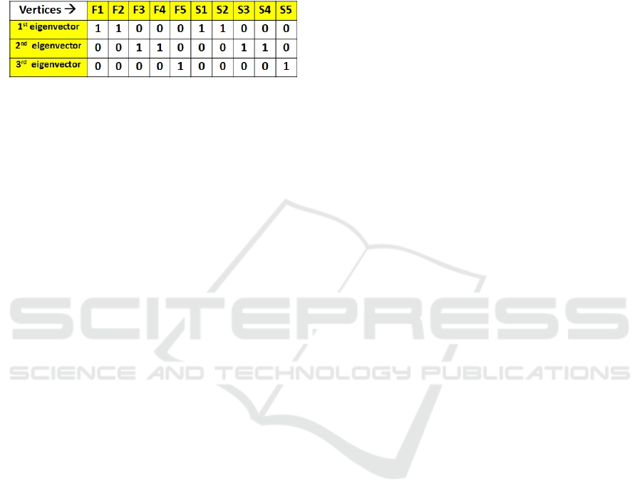
Sizes of the observer modules, the connected

components, are given by the respective

eigenvectors in Fig. 9, with functionals and structors

as follows: a- F1+S1+F2+S2+F3+S3; b-

F4+S4+F5+S5; c- F6+S6; d- F7+S7; e- F8+S8.

Design Procedure 1: Obtain Module Sizes

Set Maximal-Sparsity-Threshold;

Set Modules-Sparsity = 0;

Obtain Bipartite-Graph of Software System;

While

(Modules-Sparsity > Maximal-Sparsity-Threshold) do

{ Obtain Laplacian Matrix from Bipartite Graph;

Calculate Laplacian eigenvectors/eigenvalues;

Get eigenvectors with 0-valued eigenvalues;

Obtain Modules from these eigenvectors;

Calculate Modules-Sparsity;

If (Modules-Sparsity > Threshold)

Split Module: erase edge of Bipartite-Graph;

Save list of erased ed

;

}

Linear Software Models: Modularity Analysis by the Laplacian Matrix

105

Figure 8: Observer Laplacian Matrix – Laplacian rows and

columns are labelled with all the graph vertices of Fig. 7.

Adjacency values in the top-right quadrant are identical to

the Modularity Matrix and also reflected in the bottom-left

quadrant. Degree values appear in the Laplacian diagonal.

Figure 9: Observer Laplacian Eigenvectors – These are 5

eigenvectors corresponding to 5 zero-valued eigenvalues.

5.3 Abstract System with Outlier:

Modularity Matrix and Bipartite

Graph

The second case study is an abstract system with

unnamed structors and functionals. An outlier

element was added to the Modularity Matrix,

coupling two modules. We follow Design Procedure

1 in section 4.4 to find the modules and the outlier.

The abstract system Modularity Matrix in Fig. 10

has 3 modules and an added outlier, a 1-valued

matrix element outside the modules. Its undirected

Bipartite Graph is shown in Fig. 11.

Figure 10: Abstract System with Outlier Modularity

Matrix – The matrix has 3 modules (light blue filled). An

added outlier in row F2, column S3, (dark blue

background), couples the top-left and middle modules.

Figure 11: Abstract System with Outlier Bipartite Graph –

There are 3 modules (light blue background). The outlier

is represented by a dashed (red) line linking the vertex S3

to vertex F2, thereby coupling M1 with the M2 module.

Figure 12: Abstract System with Outlier Laplacian Matrix

– The outlier is represented by a dark (blue background) in

the Adjacency values, and by (red) 3 degree digits.

5.4 Abstract System with Outlier:

Laplacian Matrix and Eigenvectors

The Laplacian of the abstract system, shown in Fig.

12, is obtained from the undirected Bipartite Graph.

Eigenvectors fitting zero-valued eigenvalues, in

Fig. 13, are just two: a- a module of size 4, obtained

from the top-left and middle modules coupled by the

outlier; b- another of size 1, in the bottom-right.

Figure 13: Abstract System with Outlier eigenvectors –

There are just 2 modules. In the 1

eigenvector the outlier

couples two modules of size 2 into a larger module with 4

structors and 4 functionals.

By Design Procedure 1 in section 4.4, we

calculate the modules’ Sparsity. The bigger module

has 4 Structors (S1, S2, S3, S4) by the 1

eigenvector, due to the “outlier” connection seen in

Fig. 11. By Lemma 3 in section 4.3, one obtains:

Sparsity = 1 – (7/16) = 0.56

ICSOFT-PT 2016 - 11th International Conference on Software Paradigm Trends

106

Assuming a reasonable Maximal-Sparsity-Threshold

of 0.5 – i.e. the internal Sparsity of a module should

be low, meaning high Cohesion – the bigger module

is thus inferred to have an outlier.

We next erase an edge linking vertices S3 to F2

of the Bipartite Graph to split the module with too

big Sparsity. The new eigenvectors are in Fig. 14.

Figure 14: Abstract System without Outlier eigenvectors –

There are now three modules.

Recalculated Sparsity shows that the split

modules have high Cohesion. But erasing the edge

from S1 to F2, instead of the dashed “outlier” edge

from S3 to F2 in the Bipartite Graph in Fig. 11,

would also have reduced the Sparsity of the resulting

modules. Thus, the outlier resolution may not be

unique in algebraic terms. The software engineer

may need to apply semantic knowledge about

software components, to resolve couplings.

6 DISCUSSION

This work extended the formal meaning of software

system modules adding a new criterion, Connected

Components. One perceives that it appears in all

Linear Software Models’ representations of software

systems (Modularity Matrix, Modularity Lattice,

Bipartite Graph, Laplacian Matrix).

6.1 Evaluating Spectral Approaches

This work uses Laplacian eigenvectors fitting its

zero-valued eigenvalues to obtain number and sizes

of modules. Eigenvectors and eigenvalues were

calculated with the JAMA library (JAMA, 2016).

Previously (Exman, 2015) we used eigenvectors

of the Modularity Matrix symmetrized and weighted

by an affinity. The same results were obtained by

both approaches. They differ mainly by efficiency.

While Modularity Matrix weighting demands an

affinity definition, the Laplacian is neatly defined. A

Modularity Matrix advantage is its smaller size, just

one fourth of the corresponding Laplacian.

Ongoing research investigates the Laplacian

approach to larger software systems containing

outliers coupling diagonal blocks. We intend to

further formalize outliers’ treatment by the Fiedler

vector (Fiedler, 1973). This will better evaluate the

Laplacian approach for realistic systems design.

6.2 Main Contribution

This work shows that different spectral approaches

produce the same numbers and sizes of software

system modules. Behind diverse techniques, there is

just one single basic algebraic theory of software

system composition, viz. Linear Software Models.

REFERENCES

Baldwin, C.Y. and Clark, K.B., 2000. Design Rules, Vol.

I. The Power of Modularity, MIT Press, MA, USA.

Cai, Y. and Sullivan, K.J., 2006. Modularity Analysis of

Logical Design Models, in Proc. 21

IEEE/ACM Int.

Conf. Automated Software Eng. ASE’06, pp. 91-102,

Tokyo, Japan.

Exman, I., 2012. Linear Software Models, Extended

Abstract, in I. Jacobson, M. Goedicke and P. Johnson

(eds.), GTSE 2012, SEMAT Workshop on General

Theory of Software Engineering, pp. 23-24, KTH

Royal Institute of Technology, Stockholm, Sweden.

Video site:

http://www.youtube.com/watch?v=EJfzArH8-ls

Exman, I., 2013. Linear Software Models are Theoretical

Standards of Modularity, in J. Cordeiro, S.

Hammoudi, and M. van Sinderen (eds.): ICSOFT

2012, Revised selected papers, CCIS, Vol. 411, pp.

203–217, Springer-Verlag, Berlin, Germany. DOI:

10.1007/978-3-642-45404-2_14

Exman, I., 2014. Linear Software Models: Standard

Modularity Highlights Residual Coupling, Int. Journal

on Software Engineering and Knowledge Engineering,

vol. 24, pp. 183-210, March 2014. DOI:

10.1142/S0218194014500089

Exman, I., 2015. Linear Software Models: Decoupled

Modules from Modularity Eigenvectors, Int. Journal

on Software Engineering and Knowledge Engineering,

vol. 25, pp. 1395-1426, October 2015. DOI:

10.1142/S0218194015500308

Fall, K., in Focus: Perspectives-US, 2016. “Four Thought

Leaders on Where the Industry is Headed”, IEEE

Software, pp. 36-39.

Fiedler, M., 1973. “Algebraic Connectivity of Graphs”,

Czech. Math. J., Vol. 23, (2) 298-305 (1973).

Gamma, E., Helm, R., Johnson, R. and Vlissides, J., 1995.

Design Patterns: Elements of Reusable Object-

Oriented Software, Addison-Wesley, Boston, MA.

JAMA, 2016. Java Matrix Package, web site:

http://math.nist.gov/javanumerics/jama/

Merris, R., 1994. "Laplacian matrices of graphs: a survey",

Linear Algebra and its Applications, Vols. 197-198,

January-February, pp. 143-176. DOI: 10.1016/0024-

3795(94)90486-3.

Ng, A.Y., Jordan, M.I., and Weiss, Y., 2001. On spectral

Linear Software Models: Modularity Analysis by the Laplacian Matrix

107

clustering: analysis and an algorithm, in: Proc. 2001

Neural Information Processing Systems, pp.849–856.

Prototype, 2016. Web site: http://www.tutorialspoint.com/

design_pattern/prototype_pattern.htm

Shokoufandeh, A., Mancoridis, S., Denton, T. and

Maycock, M., 2005. “Spectral and meta-heuristic

algorithms for software clustering,” Journal of

Systems and Software, vol. 77, no. 3, pp. 213–223.

Shtern, M. and Tzerpos, V., 2012. Clustering

Methodologies for Software Engineering, in Advances

in Software Engineering, vol. 2012, Article ID 792024

(2012). DOI: 10.1155/2012/792024

Siff, M. and Reps, T., 1999. Identifying modules via

concept analysis, IEEE Trans. Software Engineering,

Vol. 25, (6), pp. 749-768. DOI: 10.1109/32.824377

von Luxburg, U., 2007. A Tutorial on Spectral Clustering,

Statistics and Computing, 17 (4), pp. 395-416. DOI:

10.1007/s11222-007-9033-z

Wille, R., 1982. Restructuring lattice theory: an approach

based on hierarchies of concepts. In: I. Rival (ed.):

Ordered Sets, pp. 445–470, Reidel, Dordrecht,

Holland.

ICSOFT-PT 2016 - 11th International Conference on Software Paradigm Trends

108