Video based Swimming Analysis for Fast Feedback
Paavo Nevalainen
1
, Antti Kauhanen
2
, Csaba Raduly-Baka
1
,
Mikko-Jussi Laakso
1
and Jukka Heikkonen
1
1
Department of Information Technology, University of Turku, FI-20014 Turku, Finland
2
Sport Academy of Turku Region, Kaarinankatu 3, 20500 Turku, Finland
Keywords:
Athletics, Swimming, Motion Tracking, Camera Calibration, Signal Smoothing, Movement Cycle Registra-
tion.
Abstract:
This paper proposes a digital camera based swimming analysis system for athletic use with a low budget. The
recreational usage is possible during the analysis phase, and no alterations of the pool environment are needed.
The system is of minimum complexity, has a real-time feedback mode, uses only underwater cameras, is flexi-
ble and can be installed in many types of public swimming pools. Possibly inaccurate camera placement poses
no problem. Both commercially available and tailor made software were utilized for video signal collection
and computational analysis and for providing a fast visual feedback for swimmers to improve the athletic
performance. The small number of cameras with a narrow overlapping view makes the conventional stereo
calibration inaccurate and a direct planar calibration method is proposed in this paper instead. The calibration
method is presented and its accuracy is evaluated. The quick feedback is a key issue in improving the athletic
performance. We have developed two indicators, which are easy to visualize. The first one is the swimming
speed measured from the video signal by tracking a marker band at the waist of the swimmer, another one is
the rudimentary swimming cycle analysis focusing to the regularity of the cycle.
1 INTRODUCTION
This paper describes the swimming analysis system
being developed at the Impivaara public swimming
center in Turku, Finland. Starting a new site for swim-
ming analysis requires usually considerable resources
and our economical approach with 5-7ke budget for
hardware and software licenses should be of interest
to any swimming coach considering a basic comput-
erized real-time feedback at a local site.
Budget reasons forced us to use 3 cameras only
and video coverage of 18 m. Another major constraint
was to get the system up and running with no special
initial procedure and without disturbing recreational
swimmers. The system can be expanded in the future
by a fourth camera at the grey dot depicted in Fig 1.
This setup will cover the whole 25 m pool length.
We use the video image series of the light-
reflective marker on the waist of the swimmer to
record the movement of the swimmer. The marker
moves along the tracking plane, which resides 200
mm aside towards the cameras from the centerline of
the swimming lane. The distance has been chosen so
that it approximates the dimensions of the pelvis of an
average-sized adult male and female. The real move-
ment of the marker is naturally a non-planar one, but
the planar approximation is a useful first step to sim-
plify the swimmer movement analysis. The tracking
plane of swimming lane 7 is depicted in Fig. 1. The
tracking plane has c. 1 m depth at the shallow end and
c. 2 m depth in the deep end of the pool. All the cali-
bration measurements were constrained on this plane,
and the calibration result is a geometric mapping from
the image pixels to global coordinates of the tracking
plane. Two lanes with numbers 7 and 8 were cal-
ibrated. Lane 8 is used occasionally for swimming
analysis purposes, but camera views do not cover the
whole length of the tracking plane as seen in Fig. 4.
The camera positions are constrained to win-
dowsills at the sides of the pool at the depth of 560
mm. The image mapping was constructed directly in
relation to the tracking plane, and this method does
not require usual camera model, camera locations and
orientations. The stereo calibration method proved in-
ferior because of very limited overlap between cones
of visibility, see Fig. 4.
The design emphasizes the possibility to a fast
feedback. Thus there are features which are designed
to operate in real-time during the session of athletic
Nevalainen, P., Kauhanen, A., Raduly-Baka, C., Laakso, M-J. and Heikkonen, J.
Video based Swimming Analysis for Fast Feedback.
DOI: 10.5220/0005753704570466
In Proceedings of the 5th International Conference on Pattern Recognition Applications and Methods (ICPRAM 2016), pages 457-466
ISBN: 978-989-758-173-1
Copyright
c
 2016 by SCITEPRESS – Science and Technology Publications, Lda. All rights reserved
457

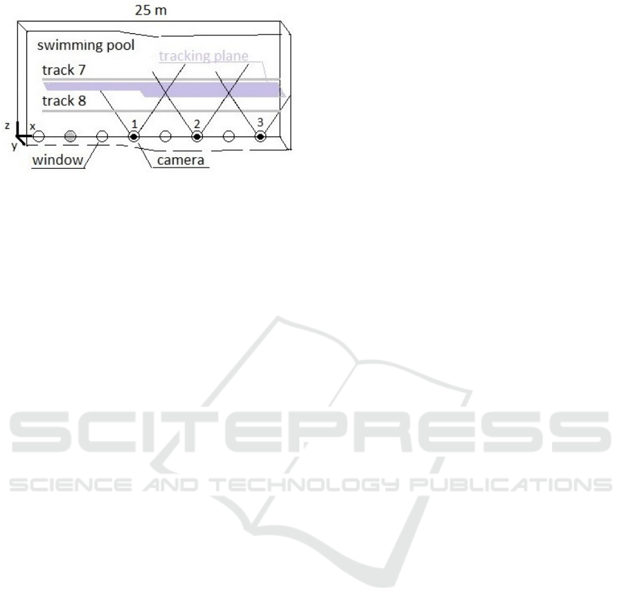
Figure 1: The general layout of the site seen from above.
The tracking plane of lane 7 is emphasized.
performance. There are also some features which are
based on the post-session phase. The forms of the
feedback implemented are:
1. Real-time marker movement tracking embedded
on the video.
2. Different performances presented side-by-side for
visual comparison and evaluation. It can be real-
time and post-session.
3. Stroke variation visualization, which is designed
so that it can be monitored by the athlete in the
pool. It can be real-time or post-session.
4. Geometric transformation of the video stream
from pixels to global coordinates. It can be real-
time or post-session.
The geometric mapping algorithm can project the
raw video to a real-time 25 fps mono-color visualiza-
tion on the tracking plane. The full quality color video
has processing speed of c. 5 fps and cannot be per-
formed in real-time. The geometric mapping will be
a crucial part for a seamless swimmer-focused view
after the swimmer detection has been implemented.
The marker tracking routine introduces both
stochastic and algorithmic noise to the signal. After
the pixel signal is transformed to global coordinates,
the signal needs to be smoothed to eliminate the noise.
The Kalman smoothing uses a basic dynamical model
of a swimmer body. Smoothing requires the record of
the whole performance as input and thus is a post-
session step.
So far the coaching routine with verbal and video
feedback has been established, but already the proce-
dure is used on weekly basis and it requires no extra
technical personnel on site.
The rest of the paper is organized as follows.
Sec. 2 is a short presentation about the current re-
search. Sec. 3 documents the architecture of the sys-
tem, tracking and swimming cycle registration. Sec. 4
presents the used in-plane calibration method in de-
tail, since this aspect is heavily dictated by the budget
limitations yet opens possibilities for future research
as well. Sec. 5 is about the real-time tracking visual-
ization.
The swimmig cycle registration and comparison
presented in Sec. 6 has been an important early facil-
ity for the coaching. The post-session analysis phase
of Sec. 7 is one adaptation to the budget limitations.
Sec. 8 summarizes the design choices made to achieve
the real-time system response. Sec. 9 has conclu-
sions and discussion about the possible future devel-
opments.
2 LITERATURE REVIEW
There are several approaches to swimming analysis.
The oldest one is using wire. (Jean-Claude, 2003)
reports about measuring the force in the wire while
some object is dragged behind, another method is
measuring the swimmer speed directly using the wire.
The mechanical method is used especially to verify
the video installments.
Video analysis is the dominant mode of perfor-
mance analysis nowadays, see e.g. a review of the
field in (Kirmizibayrak et al., 2011). A typical ap-
proach is:
• to produce the continuous video stream from mul-
tiple cameras
• and trace anchor points of the body (marked or
nonmarked) and then
• combine the acquired information to a biome-
chanical or 3D visualization model.
There are several commercial tools available,
many of them summarized in (Kirmizibayrak et al.,
2011). Typical examples are Dartfish (Dartfish, 2015)
and Sports Motion (Sportsmotion, 2015).
Wearable accelerometers are relatively new tools.
These are developing smaller and lighter, also the op-
eration time is increasing due the lower power re-
quirements and increased battery capacity. (Dadashi
et al., 2013) shows an arrangement with only one
accelerometer to record the swimming performance
over the full length of the pool. The data link is
usually radio-linked in bursts like e.g. (James et al.,
2011), or in the end of the performance, like in
(Dadashi et al., 2013).
A typical large scale system design can be found
from (Mullane et al., 2010). They provide an ex-
cellent analysis of what feedback should be provided
real-time and what at post-session phase.
Swedish Center for Aquatic Studies has AIM
(Athletes in Motion) system which can combine
views from submerged and above-water cameras,
ICPRAM 2016 - International Conference on Pattern Recognition Applications and Methods
458

see (Haner et al., 2015). The calibration process re-
sembles our approach albeit they use striped poles
while we use chessboard pattern. AIM has been de-
veloped by efforts of Chalmers and Lund Universities.
Chalmers University has a multiple accelerometer
arrangement, which is coupled with a video analysis
and a biomechanical model. Accelerometers can be
placed by suction cups to various areas of the body.
One study shows how a relatively low frequency still
provides adequate biomechanical modeling (Siirtola
et al., 2011).
Another video technique is the virtual camera
technique, where a moving viewpoint is synthetized
between two adjacent cameras. It is possible to in-
terpolate the view between stationary spots like in
(Makoto et al., 2002).
Head is a popular choice of strapping the athlet
with a sensor device. One can wear a colored cap, or
swimming glasses with an accelerometer, see (Pansiot
et al., 2010).
Relatively new approach is the video analysis
without markers (Ceseracciu, 2011). From athlete
point of view it is much less intrusive and enables au-
tomation of the analysis process.
The trend in research seems to be towards 3D
visualization and increasing usage of biomechanical
models. Actual analysis is quite developed and re-
maining goals are at quick performance feedback and
well visualized and conceptually simple performance
measures.
As a summary, existing systems are well-
developed and serve the coaching activities well. Of-
ten the implementation is rather involved requiring
technical assistance, set-up times and high initial and
running costs. Our aim was to produce a cheap and
simple non-intrusive alternative with stable basis for
further improvement.
3 SYSTEM DESCRIPTION
The system consists of:
• one 2-core 3.2 GHz 64 bits computer with. 2 TB
of disc space
• 3 permanently placed 50 fps cameras at the side
wall of the 25 m pool. The maximum image size
is 750 × 2044. The camera placement is dictated
by the construction of the pool.
• one movable extra camera for above-water usage
and one movable underwater camera. Usage of
the extra cameras is just for visual observation and
verbal feedback only.
• movement marker and band at the hip of the
swimmer.
The cameras and computer record and store over 50
fps high resolution digital video in uncompressed for-
mat. The image size is 750 × 2044 pixels. An indi-
vidual pixel of the geometrically transformed image
corresponds to 4.0 × 4.0 mm
2
and 2.3 × 2.3 mm
2
on
lanes 7 and 8, correspondingly.
The uncompressed data from three cameras
amounts to about 1GB for a 10 second clip. All cam-
eras are synchronized so that they capture images at
the same time. The time stamps are stored in the video
files and they can be used in determining how to stitch
the tracking results.
Marker tracking algorithm utilizes OpenCV pack-
age (Bradski, 2000). Camera calibration was done
with self-developed software.
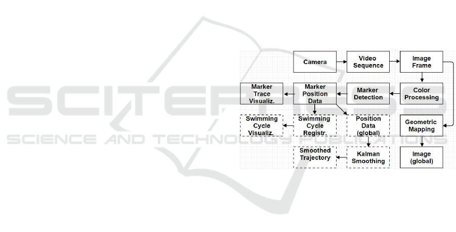
Process is divided to real-time and post-session
phases. Figure 2 illustrates the various steps of the
process. The recorded video is stored in a raw uncom-
pressed file format specific to the camera manufac-
turer and is later accessed by the post-session phase.
Figure 2: The processes and data flow. Post-session steps
are indicated by the dashed outline.
4 CAMERA CALIBRATION
Camera calibration is a preliminary measurement pro-
cess delivering either the camera model (mapping
from pixels to normal vectors of the pinhole camera
idealization) or the direct geometric mapping from
pixels to global positions.
Three calibration methods, stereocamera
(Bouguet, 2008), mono-camera (Bouguet, 2008)
and our own direct planar calibration were tested.
The stereo-calibration is an industry standard
method since it is able to produce depth information
(3D) and is not limited to the tracking plane G of
Fig. 1. It calibrates the full camera view just like the
mono-camera method. It also provides an early qual-
ity check in the form of relative camera positions de-
Video based Swimming Analysis for Fast Feedback
459

picted in Fig. 3. The position error was c. 85
mm even after the best possible calibration measure-
ments described in (Bouguet, 2008).
Figure 3: The camera positions from stereo-calibration.
Reason for the low accuracy is the difficult geom-
etry of the camera positions dictated by the location of
the windowsills of the pool, see Fig. 1. The amount of
overlap of the camera views is only c. 22%, see Fig. 4
with refraction included, whereas the overlap ratio in
a usual stereo calibration analysis is above 50%.
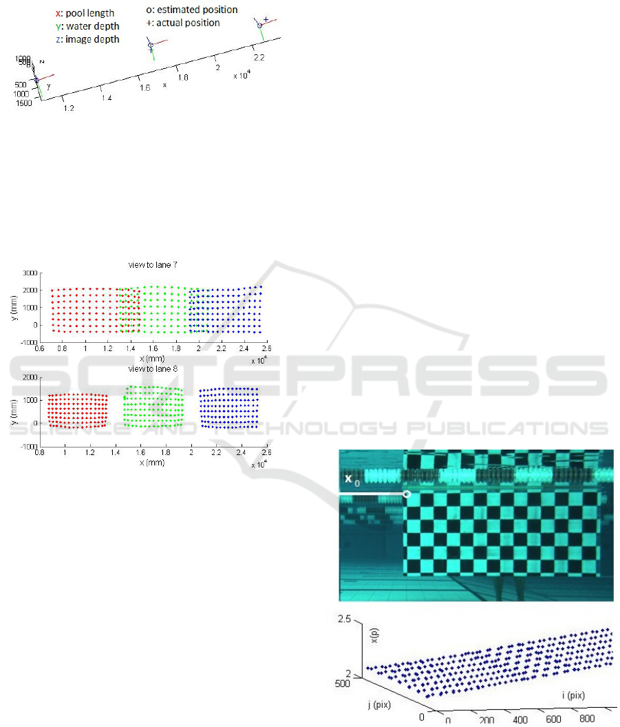
Figure 4: The area of visibility per each camera on the
tracking plane. Colors (red/green/blue) correspond to cam-
eras (1/2/3). Only c. 22% of the view is overlapping at lane
7. The lane 8 is closer to cameras, and there is no overlap-
ping anymore.
The small overlap also rules out the homography
approach described in (Chum et al., 2005) applied to
all the sample points at the whole tracking plane at
once. Otherwise that method would have been excel-
lent, since it is able to use the expected location errors.
The mono-camera approach is very close to
stereo-calibration, except the location and orientation
of each camera is a separate subject of the match-
ing process, when a fit is made to the tracking plane
data. The mono-camera method is also close to the
direct planar calibration presented in Sec. 4.1. The
main difference is that the direct calibration requires
no camera model (not even the camera location) and
that the mapping from pixels to global locations can
be arbitrarily chosen. The mono-camera calibration
produces better mapping quality at the image borders
than the direct planar calibration. The difference is
aesthetic only, since the accurate zone of the direct
calibration can be made large enough to accommo-
date all the swimmer motions. Also the mono-camera
approach has been omitted from this presentation.
The stereo and mono calibrations were done with
Matlab Camera Calibration Toolbox, see (Bouguet,
2008). The theory of the toolbox is given at (Zhang,
1999) and (Heikkil
¨
a and Silven, 1997).
The most accurate method was the direct planar
calibration proposed in Sec. 4.1. This method can be
categorized as an ad hoc approach answer to two con-
straints: sparsely placed camera array and potential
for real-time video transformation. Nearest reference
is (Luo et al., 2006), which uses a camera model and
requires the co-planarity of the camera image plane
and the tracking plane. Our method requires no cam-
era model. The direct planar method is presented in
the following.
4.1 Direct Plane Calibration
The geometric calibration was done for lanes 7 and
8 of ten available lanes. The calibration data for the
direct method was gathered by floating a calibration
chessboard along the surface at the tracking plane and
recording its position at each picture, see Fig. 5. The
chessboard had buoys at the top and weight at the bot-
tom. The global position x
0
of the board was mea-
sured within 10 mm accuracy std.
Figure 5: Direct calibration on the tracking plane. Above:
an individual x
0
position of the calibration board at camera
2 view. Below: the cumulated observation set U of camera
1 consisting of corner point pixels p and global positions
g ∈ R
3
from all images of lane 7 at camera 1. Only the x
component of the global position g depicted.
ICPRAM 2016 - International Conference on Pattern Recognition Applications and Methods
460

To ease the presentation, some definitions are
needed. An image I = (P,J) of size n × m is a pair of
set of pixels p ∈ P = [1, n] × [1,m] ⊂ Z
2
+
and their in-
tensities J = { j(p)|p ∈ P}, where an individual pixel
p has intensity j(p). Images come in three varieties,
source images I
s
= (P
s
,J
s
), geometrically transformed
target images I
t
= (P
t
,J
t
), and calibration images.
The tracking plane G = {g ∈ R
3
| (g − g
G
) · n
G
=
0} is defined by one insident point g
G
= (0, 0, z
0
)
T
,
where z
0
= 5050 mm in case of lane 7. The 200 mm
aside of the center of the swimming lane. The normal
vector n
G
is a unit vector aligned with the global z
axis. The marker is assumed to move along this track-
ing plane. Fig. 1 depicts the tracking plane G and the
global coordinates x,y,z.
A chessboard corner pixel and its corresponding
global positions form a measurement pair (p,g) ∈ U.
The calibration data set U is cumulated over all cali-
bration images. One measurement image is depicted
at the upper part of Fig. 5. The lower part shows the
measurement set U (only x component of g shown).
The pixel samples of U cover only a part of the im-
age pixels P whereas the end result of the direct plane
calibration maps all pixels of the source image onto
the tracking plane P
s
→ G. In that sense this is an
interpolation problem.
In the following, only the mapping of the x com-
ponent is detailed. The y component has a similar
treatment and is omitted for brevity. There would
be some advantage to use a coupled mapping p →
(x,y) e.g. a mono-camera model for interpolation but
even this rudimentary approach with two independent
mappings produced encouraging results.
A piecewise bilinear smoothing function:
x = f (p, α
∗
x
) (1)
with shape parameters α
∗
x
∈ R
d
and automatic tiling
heuristics is used to set a map p → x from pixels p to
the global coordinate x. The shape parameter dimen-
sion d ∈ N
+
varies case by case because of the imple-
mentation (D’Errico, 2006) but is in this application
d ≈ 80. The regularization parameter λ
x
∈ R
+
con-
trols the smoothness. The definition below uses func-
tionals A
x
for error penalty and B for non-smoothness
penalty:
α
∗
x
= argmin
α
A
x
( f (.,α)) +λ
x
B( f (.,α))
A
x
( f (.,α)) =
∑
(p,g)∈ U
( f (p,α) − x)
2
(2)
B( f (.,α)) =
∑
(p,g)∈ U
(mean
q∈N
p
f (q,α) − f (p,α))
2
In the above, N
p
is the set of neighboring pix-
els of p at pixel radius r = 2. The function f (.,.)
is implemented as Matlab gridfit.m with ’bilinear’
and ’laplacian’ options, see (D’Errico, 2006). Val-
ues λ
x
= 120, λ
y
= 180 were chosen to keep the non-
smoothness measure B(.)/A(.) tolerable.
4.2 Precomputed Mapping
Let us combine Eqs. 2 and 1 for further treatment.
The source image pixels p
s
are mapped to tracking
plane G by:
F
s
(p
s
) = ( f (p
s
,α
∗
x
), f (p
s
,α
∗
y
),z
0
) ∈ G, p
s
∈ P
s
(3)
The image of I
s
on G is now F
s
(I
s
). The target image
I
t
is mapped to tracking plane G by:
F
t
(p
t
) = g
0
+ γ


0 1
1 0
0 0


p
T
t
∈ G, p
t
∈ P
t
(4)
The target image pixel size γ = 4.0 mm for lane 7 and
γ = 2.3 mm for lane 8. Image location g
0
is specific
for each camera view on each swimming line. Pixel
p = (i, j) has row and column indices as depicted in
Fig. 6. It is now possible to interpolate the intensity
value of p
t
using Shepard interpolation of Eq. 6 at the
tracking plane G.
First, some definitions. Let |P
t
| be the number of
pixels in the image I
t
and M ∈ N
|P
t
|×4
+
be a reference
pixel matrix. One row M
p
t
.
specified in Eq. 5, holds
4 reference pixels from P
s
for a pixel p
t
∈ P
t
. The
nearest neighbor operator NN
k
(x,X) selects k nearest
neighbors of x from a set X. Sets are treated as vec-
tors whenever there is a unique enumeration of the
set. The location of p
t
is g
t
. N
t
is the set of 4 nearest
neighbors of the sourcce image locations ar G.
g
t
= F
t
(p
t
)
N
t
= NN
k
(g
t
,F
s
(P
s
)) ⊂ G, k = 4
M
p
t
i
= F
−1
s
(N
ti
) ⊂ P
s
, i = 1...4 (5)
W
p
t
i
= {s(kg
i
− g
t
)k) | g
i
∈ N
t
}
0
, i = 1..4 (6)
s(r) = 1/ max(r, 0.05 mm)
where W ∈ R
|P
t
|×4
+
is a radial interpolation weight ma-
trix with a correspondence to same indexing as ma-
trix M. Function s(r) is the radial weight used. The
normalization in Eq. 6 happens by L
1
norm: w
0
=
w/
∑
i
|w
i
| for a general weight row w.
Considering pixel intensities J
t
and J
s
as vectors
indexed by pixels, the transformation becomes:
J
t
(p
t
) :=
k
∑
i=1
J
s
(M
p
t
i
)W
p
t
i
(7)
By selecting k = 1 one gets the real-time transforma-
tion:
J
t
(p
t
) := J
s
(M
p
t
1
) (8)
Video based Swimming Analysis for Fast Feedback
461

Eq. 8 corresponds to the Nearest Neighbor refer-
encing which can be computed at 25 fps (measured
with Matlab). The case k = 4 of Eq. 7 can be com-
puted at 5 fps and thus is not usable in real-time. The
quality of k = 1 case is adequate to a video stream,
see Fig. 6. If quality par the original is required, one
can use Eq. 7. The balance between speed and quality
can be tuned further by choosing k = 2 or k = 3.
The geometric image mapping is efficient and
simple, see Eqs. 8 and 7. The formulation used also
makes it possible to combine the three separate video
signals accurately to one single video. This feature
will be implemented when an automated swimmer
targeting is added to the system.
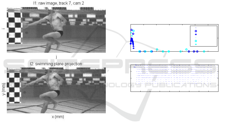
Figure 6: Quality of the fast mapping, a detail at the oppo-
site wall. Above: the source image I
s
with pixel coordinates
i and j. Below: the target image I
t
with global coordinates
x and y.
4.3 Error analysis
The measurement points U in Fig. 5 are in approx-
imate horizontal rows. There is c. 150 mm vertical
gap between rows and c. 50 mm average horizontal
distance between points. This requires the interpolant
to have rather high penalty for non-smoothness.
The pixel detection was done with Matlab de-
tectCheckerBoard.m function, theory of which is con-
tained in (Zhang, 2000). The pixel detection error
is p ≈ (1,1). The mechanical placement accuracy of
the measured points (p,g) ∈ U is ∆g ≈ (10,10,10 +
0.01z)
T
mm as an approximate std. The error is un-
biased and the final accuracy of F
s
(p
s
) is much better.
A pixel-wise geometric mapping error measure
e(p) is formulated by Eq. 9 and depicted at Fig. 7:
e(p) = kg − F
s
(p)k, (p,g) ∈ U (9)
Since the sample set U is of rather good quality and
since the function F
s
is rather smooth, the error stays
almost constant even if the tuning of the shape param-
eters α
x
,α
y
in Eq. 2 is subjected to cross-validation
over subsets of U. The error is largest in occasional
points at the border and grows rapidly when extrap-
olating. The border areas are seldom occupied by a
swimmer, though, and the problem is more of aes-
thetical nature. The border error can be eliminated in
the future by applying a different interpolant instead
of one in Eq. 3.
0 5 10 15 20 25 30
10
0
10
2
10
4
Geometric error distributions, tracks 7−8, cams 1−3
||∆ g|| (mm)
freq.
std(Delta g): 1.68 (mm) (= 0.6 pixels)
2.05 2.1 2.15 2.2 2.25 2.3 2.35 2.4 2.45 2.5
x 10
4
0
500
1000
1500
2000
x (mm)
y (mm)
geom. error, t8,c3
lane 7 cam 1
lane 7 cam 2
lane 7 cam 3
lane 8 cam 1
lane 8 cam 2
lane 8 cam 3
Figure 7: The geometric mapping error e(p), p ∈ P
s
defined
by Eq. 9. Large errors happen occasionally at the borders of
the sampled area U.
5 REAL-TIME TRACKING
The swimmer tracking method is based on marker
tracking using the blob tracking facilities of OpenCV
(Bradski, 2000). The marker is placed on a colored
flexible band worn by the athlete in order to improve
accuracy and reduce noise. The band is selected and
installed so that it will not hinder the performance of
the swimmer. The yellow color of the band is chosen
to increase its visibility and identifiability in the envi-
ronment. The band can be occluded by the swimmer’s
hand, or by bubbles in the water.
The color of the band is selected based on the
color hue distribution of the environment. Tests on
the site showed that the environment colors (water,
swimmer, light, walls, etc) are between the interval
ICPRAM 2016 - International Conference on Pattern Recognition Applications and Methods
462

90
◦
− 270
◦
, leaving the rest of the hue circle open.
We selected a yellow color band. The choice leaves
room for one or two extra markers, if needed in some
future analysis.
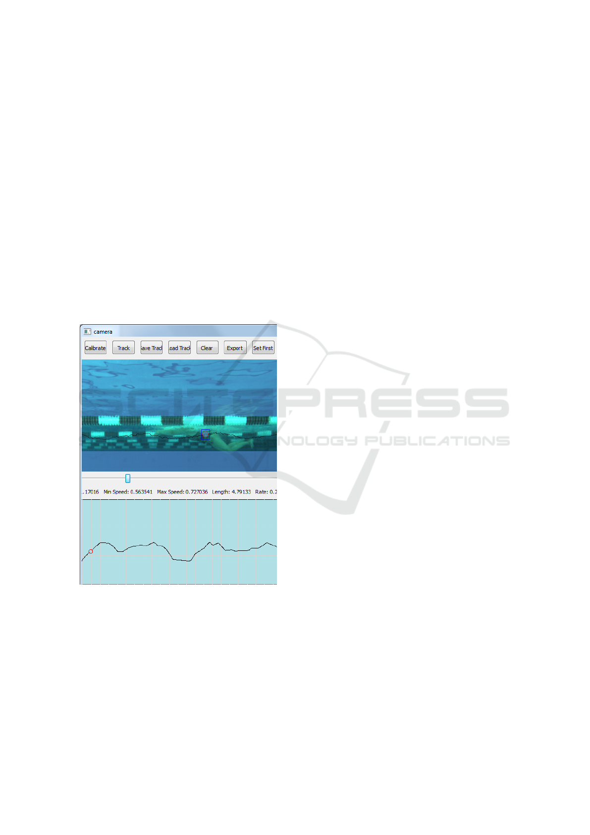
The pixel trajectory of the marker is being visu-
alized for the user in real-time, see Fig. 8. The pixel
trace is then being mapped to global coordinates on
the tracking plane using the geometric mapping de-
scribed in Sec. 4. Tracking performs well with the
current 50 fps speed allowing the real-time rendering.
The visualized points are referring to image pixel
coordinates and are not suitable for speed analy-
sis. The swimmer speed is calculated by converting
these points using the geometric mapping described
in Sec. 4.
The real-time swimmer trace is provided as an
overlay curve at the video area, see Figure 8. The
current frame position is highlighted. The recorded
session can be replayed immediately.
Figure 8: Presenting the tracking results to the user. The
emphasised square is for the user only and it does not cor-
respond to the tracking plane. The track is based on pixel
information for reducing response time.
6 SWIMMING CYCLE
REGISTRATION
A swimming cycle is the state history over a time in-
terval during which the swimmer state returns rela-
tively close to the initial state. The maximum per-
formance requires rather monotonic strokes, yet the
rhythm may vary based on metabolical optimum. De-
tecting the regularity of swimming strokes is of im-
portance. Cycles seem to have a distinctive decelera-
tion phase just before each hand stroke. This enables
a simple cycle registration by finding a local spike
heuristically in phase signal at times t
i
∈ R
+
, i ∈ N
+
.
Using a peace-wise linear parameter τ:
t(τ) = t
i
(τ−i)+t
i+1
(i+1 −τ), i = bτc, τ ∈ R
+
(10)
one can compare the shapes of two cycles i and j di-
rectly in a duration-invariant way on their own relative
time scale t
i
+ τ. Let us define the duration of a cycle
i as T
i
= t
i+1
− t
i
. Now, the dissimilarity d
i j
between
two cycles i and j can be defined:
d
i j
= [
Z
1
0
(v
x
(t(i + τ)) − v
x
(t( j + τ)))
2
dτ]
1/2
+
+ λ|T
i
− T
j
| (11)
The horizontal velocity v
x
in Eq. 11 is based on pixel
information with a moving average smoothing, since
we noticed the raw pixel signal is enough for the cycle
detection. The last summand of Eq. 11 sets a weight
on the duration difference between two strokes. The
duration difference penalty is open to experimenta-
tion, currently we use value: λ = 4. We have used
the vertical velocity v
x
(t) as the target signal for sim-
ilarity analysis. The target signal could be also the
horizontal velocity or a vector combination of both,
in which case a vector norm should be used in Eq. 11.
The swimming cycle registration is a post-session
process, which will be implemented as a real-time
feature in the future. A similarity matrix is cumu-
lated from last few strokes (last 5 in cases depicted
in Fig. 9). The visualization is designed to be seen
directly from the pool. The colors are scaled so
that black is a serious deviation from allowed, white
means identical strokes. Each stroke is compared to
others and no judgement is made towards the quality
of the swimming performance in general. The gray-
scale used is an arbitrary choice at the moment.
7 POST-SESSION PHASE
The post-session phase occurs when there is a pause
in the athletic performance. First, the recorded video
is stored on the hard disc. The trainer opens the video
file with the tracking software and it is able to provide
feedback to the coach and swimmer in a reasonable
time (at most a few minutes).
The software allows the overlaying of multiple
tracking results of different athletes. The trainer can
Video based Swimming Analysis for Fast Feedback
463

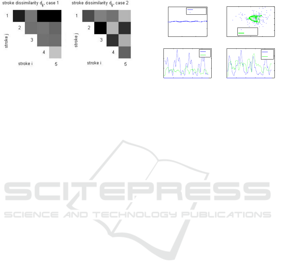
Figure 9: Swimming stroke regularity visualization. Rows
and columns are individual strokes. White means zero dif-
ference and black a difference d
i j
= 0.2 m/s.
use these data overlays to compare a trainee with a
reference (trained) swimmer performance.
The speed graphs acquired by geometric trans-
form of the original pixel trace are displayed in a sep-
arate area of the screen under the video frame. The
graphs span the whole observed length.
A number of quantitative measures are displayed
on the current swimmer performance, like aver-
age speed, distance, time, minimum and maximum
speeds. A specific time period can be highlighted
in the speed graph, to restrict the numeric display to
measurements on this area.
There will be further experiments on visualizing
various swimming characteristics. Preference will be
given to the real-time feedback.
7.1 Kalman Smoothing
Kalman smoothing (J. Hartikainen and and S
¨
arkk
¨
a,
2011), is applied to pixel trace to get smoothed plots
of the position and velocity components over time.
Fig. 10 depicts the smoothed position and velocity
history. Further swimming style analysis and move-
ment registration operations can be based on this sig-
nal.
The marker observations are described as com-
ing from a linear dynamical system of Eq. 12 with
Gaussian noise w ∼ N(0, dσ
2
x
,σ
2
y
c) as the driving
force component. Our numerical choice was: σ
x
=
10 N, σ
y
= 20 N. Other constants of Eq. 12 are spec-
ified in Eq. 13:
m
¨
g(t) + c
˙
g(t) + k g = w(t) (12)
The system is further discretized to given non-regular
observation times and transformed to a discrete-time
linear dynamical model with Gaussian noise term, see
details from (J. Hartikainen and and S
¨
arkk
¨
a, 2011).
The numerical values of the swimmer model of
Eq. 12 are chosen for an average swimmer, and
the dampening parameters approximate the observed
0 2 4
−2
−1
0
1
2
x(t) (m)
y(t) (m)
Position
Smoothed
Measured
0 0.5 1 1.5 2
−1.5
−1
−0.5
0
0.5
1
v
x
(t) (m/sec)
v
y
(t) (m/sec)
Velocity
Smoothed
Measured
0 1 2 3 4 5
0
0.01
0.02
0.03
Moving deviation
t (sec)
location deviation (m)
σ x
σ y
0 1 2 3 4 5
0
0.1
0.2
0.3
0.4
t (sec)
velocity deviation (m/s)
Moving deviation
σ v
x
σ v
y
Figure 10: The smoothed position and velocity of the
marker tracking. Above: Measured and smoothed signals.
The current tracking brings large procedural noise compo-
nent to velocity. Below: The moving deviation estimates.
Only one camera view was used in this demonstration.
speed resistance of swimming. The model will be im-
proved later e.g. using Gaussian process formulation
instead of Kalman, adding more biomechanical au-
thentity to the model and physically interesting latent
forces, see e.g. (Hartikainen et al., 2012):
m = I
2
× 60 kg (mass)
c = d11.7 16.3c kg/s (dampening) (13)
k =

0 1
1 2

× 0.05 kg/s
2
(spring)
The average error (std.) of the procedure is at the mo-
ment ∆x = 0.018 m, ∆y = 0.008 m, ∆v
x
= 0.2 m/s,
∆v
y
= 0.2 m/s for positions and velocities along x and
y axes. Improvements will be made by applying a bet-
ter tracking method less sensitive to bubbles.
Kalman smoothing is a post-processing task, too.
8 SYSTEM PERFORMANCE
A principal objective of the system is to provide im-
mediate trainer feedback. To achieve that, the imple-
mentation is based on the following principles:
• The frames are processed and tracked in their
uncalibrated shape (containing all camera distor-
tions, refraction etc.). The physical meaning for
the tracking signal can be attached only after the
geometric mapping, which is a postprocessing
step, see Fig. 2.
• The tracked area is limited manually, see the high-
lighted area in Fig. 8. Usually swimmers occupy
only a narrow band on the screen. Limiting the
tracking to this area of interest reduces compu-
tation significantly. At the moment, the tracking
box (see Fig. 8) is selected manually, but there
ICPRAM 2016 - International Conference on Pattern Recognition Applications and Methods
464

will be few prerecorded tracking areas for differ-
ent swimming styles in the future.
• The dissimilarity measure of Eq. 11 is also based
on the raw pixel information. The formula is com-
putationally cheap, and it has to be evaluated on
a separate processor once when swimmer passes
a camera. Full real-time indicator will be imple-
mented when a second computer and a monitor
will be added to the system.
• The geometric mapping of video images uses re-
duced quality to deliver real-time performance.
• Seamless (combined from 3 cameras) geomet-
rically accurate visualizations like video, stroke
regularity indication and physical speed analysis
are all left as a post-processing step. At this phase,
the geometric mapping has been done to images
and data already.
9 CONCLUSIONS
We have presented a simple video-based swimming
analysis system which is easy to install, is of low cost
and is simple to calibrate without any technical assis-
tance. It can be installed to a wide variety of pool
types. It is maintenance free and based on our experi-
ence so far, it can be operated by one person only. In
ordinary use no technical assistance is needed.
The proposed system provides swimming speed
analysis and instant visual feedback. The system is a
good basis for further expansion e.g. with swimming
gait analysis, biomechanical modeling etc.
The current system can be easily upgraded by a
fourth camera at the location indicated by a grey cir-
cle in Fig. 1. The video monitoring would then span
whole the pool length. A second video screen will be
added in the future to serve the athletes better.
There are many off-the-shelf analysis systems
with a wide spectrum of functionality available today.
Usually these systems are much more complex and
expensive than one presented here. Our choice was to
implement the real-time pixel trace of the marker and
swimming cycle regularity visualization.
The tracking system needs to be improved in the
near future. At the moment it falls off-the-track too
often, especially when a hand moment occludes the
already lost marker.
The current system has been used by Finnish na-
tional swimming teams both on senior and junior level
since autumn 2014. Automated tracking has made it
possible to give faster and more accurate feedback to
athletes. Thus it has been possible to test a large num-
ber of athletes in relatively short time during national
team camps, when previously only a few of the top
swimmers were able to get the service due to time in-
vestment required using the older version of the sys-
tem. According to national team coach the system
has been a major asset in developing technical skills
of national team athletes. The findings have also been
used in national coaches’ education to provide insight
into swimming performance.
The proposed direct planar calibration method
used is aimed for efficient real-time video stream
transformation. The efficiency is possible due to the
restriction to 2D tracking plane projection only. There
is potential for the same formulation to be generalized
for 3D motion capture at the overlapping view zones
(2 × 2 m at the current system, 3 × 2 m after one cam-
era will be added). The proposed calibration method
may be of use in other applications where conditions
in camera placement rule the stereo-calibration out
and where planar observations suffice.
The most important future goals are a reli-
able markerless tracking and implementing a record
database with automated input from the site and a sup-
port for rudimentary searches and comparisons.
The swimming gait registration based on the pro-
file shape of the body of the swimmer is a potential
development.
Automated detection of different phases of the
swimming performance remains the last goal. It is
the hardest since there are a lot of different swimming
styles each with somewhat differing phases, and fe-
male and male swimming costumes differ.
ACKNOWLEDGEMENTS
The project is a joint venture of University of Turku
IT department and Sports Academy of Turku region
and it has been funded by city of Turku, National
Olympic Committee, Finnish Swimming Federation,
Urheiluopistos
¨
a
¨
ati
¨
o and University of Turku.
REFERENCES
Bouguet, J. Y. (2008). Camera calibration toolbox for mat-
lab.
Bradski, G. (2000). Opencv. Dr. Dobb’s Journal of Software
Tools.
Ceseracciu (2011). New frontiers of markerless motion cap-
ture: application to swim biomechanics and gait anal-
ysis. PhD thesis, Padova University.
Chum, O., Pajdla, T., and Sturm, P. (2005). The geometric
error for homographies. Comput. Vis. Image Underst.,
97(1):86–102.
Video based Swimming Analysis for Fast Feedback
465

Dadashi, F., Millet, G., and Aminian, K. (2013). Iner-
tial measurement unit and biomechanical analysis of
swimming: an update. Sportmedizin, 61:21–26.
Dartfish (2011-2015). Dartfish video analysis tool.
http://www.sportmanitoba.ca/page.php?id=116.
D’Errico, J. (2006). Surface fitting using gridfit. Technical
report, MATLAB Central File Exchange.
Haner, S., Sv
¨
arm, L., Ask, E., and Heyden, A. (2015).
Joint under and over water calibration of a swimmer
tracking system. In Proceedings of the International
Conference on Pattern Recognition Applications and
Methods, pages 142–149. ScitePress.
Hartikainen, J., Sepp
¨
anen, M., and S
¨
arkk
¨
a, S. (2012). State-
space inference for non-linear latent force models with
application to satellite orbit prediction. CoRR.
Heikkil
¨
a, J. and Silven, O. (1997). A four-step camera cal-
ibration procedure with implicit image correction. In
Proc. IEEE Conference on Computer Vision and Pat-
tern Recognition, pages 1106–1112.
J. Hartikainen and, A. S. and S
¨
arkk
¨
a, S. (2011). Optimal
filtering with kalman filters and smoothers, a manual
for the matlab toolbox ekf/ukf. Technical report, Dept.
of Biomedical Eng. and Comp.Sci., Aalto University
School of Science.
James, D. A., Burkett, B., and Thiel, D. V. (2011). An unob-
trusive swimming monitoring system for recreational
and elite performance monitoring. In Procedia Engi-
neering, 5th Asia-Pacific Congress on Sports Technol-
ogy (APCST), volume 13, pages 113–119.
Jean-Claude, C., editor (2003). Biomechanics and Medicine
in Swimming IX. IXth International World Symposium
on Biomechanics and Medicine in Swimming, Uni-
versit
´
e de Saint-Etienne.
Kirmizibayrak, J., Honorio, J., Xiaolong, J., Mark, R., and
Hahn, J. K. (2011). Digital analysis and visualization
of swimming motion. The International Journal of
Virtual Reality, 10(3):9–16.
Luo, H., Zhu, L., and Ding, H. (2006). Camera calibra-
tion with coplanar calibration board near parallel to
the imaging plane. Sensors and Actuators A: Physi-
cal, 132:480486.
Makoto, H. S., Kimura, M., Yaguchi, S., and Inamoto, N.
(2002). View interpolation of multiple cameras based
on projective geometry. In In: International Workshop
on Pattern Recognition and Understanding for Visual
Information.
Mullane, S. L., Justham, L. M., West, A. A., and Conway,
P. P. (2010). Design of an end-user centric information
interface from data-rich. In Procedia Engineering,
volume 2, pages 2713–2719. 8th Conference of the
International Sports Engineering Association (ISEA).
Pansiot, J., Lo, B., and Guang-Zhong, Y. (2010). Swimming
stroke kinematic analysis with bsn. In Body Sensor
Networks (BSN), 2010 International Conference on,
pages 153–158.
Siirtola, P., Laurinen, P., Roning, J., and Kinnunen, H.
(2011). Efficient accelerometer-based swimming ex-
ercise tracking. In IEEE Symp. on Computational In-
telligence and Data Mining (CIDM), pages 156–161.
IEEE.
Sportsmotion (2011-2015). motion analysis system.
http://www.sportsmotion.com/.
Zhang, Z. (1999). Flexible camera calibration by viewing a
plane from unknown orientations. In in ICCV, pages
666–673.
Zhang, Z. (2000). A flexible new technique for camera cali-
bration. In IEEE Transactions on Pattern Analysis and
Machine Intelligence, volume 22, page 13301334.
ICPRAM 2016 - International Conference on Pattern Recognition Applications and Methods
466