Fine-Grained Prediction of Cognitive Workload in a Modern Working

Environment by Utilizing Short-Term Physiological Parameters

Timm H

ormann, Marc Hesse, Peter Christ, Michael Adams, Christian Menßen and Ulrich R

uckert

Cognitronics and Sensor Systems Group, CITEC, Bielefeld University, Bielefeld, Germany

Keywords:

Fine-Grained, Cognitive Workload, Stress, Heart Rate, Electrodermal Activity, Tablet Computer, Human

Machine Interaction, Industry 4.0.

Abstract:

In this paper we present a method to predict cognitive workload during the interaction with a tablet computer.

To set up a predictor that estimates the reﬂected self-reported cognitive workload we analyzed the information

gain of heart rate, electrodermal activity and user input (touch) based features. From the derived optimal

feature set we present a Gaussian Process based learner that enables ﬁne-grained and short term detection of

cognitive workload. Average inter-subject accuracy in 10-fold cross validation is 74.1 % for the ﬁne-grained

5-class problem and 96.0 % for the binary class problem.

1 INTRODUCTION

Today’s modern working environments are increas-

ingly challenging for the employees. As one example

the concept of ”Industry 4.0” sketches the design of

new ﬂexible working environments, in which employ-

ees are constantly confronted with new requirements.

This implies manufacturing processes with very small

lot sizes, which will result in a higher diversity of

working processes. It forces the employees to be

highly ﬂexible and to adapt rapidly to changing work

tasks. For instance, the employees will have to mem-

orize and apply new knowledge more often (Botthof

and Hartmann, 2015). Therefore, adaptive Human-

Machine-Interaction (HMI) becomes more important.

Especially by means of the implementation and uti-

lization of adaptive assistive systems, which shall be

used to guide an employee through a new and unfa-

miliar task (Wallhoff et al., 2007). With the ability

to balance the cognitive workload (CW) of a speciﬁc

task, the ergonomic design of working tasks could be

improved. This makes the prediction of CW a key

factor towards human centric design, concerning the

development of adaptive HMI and adaptive assistant

systems. (Rouse et al., 1993) (Wallhoff et al., 2007)

To fulﬁll the requirement of adaptability, an as-

sistive system needs to know the human users’ cog-

nitive capacity. Therefore, in order to adjust corre-

spondingly to the user’s needs, it is important to pre-

cisely model the user’s perceived CW. The goal is to

balance the complexity of a given task. This is be-

cause, on the one hand, if the user is not sufﬁciently

assisted, it might lead to mistakes. But on the other

hand, if the user feels unchallenged, it might decrease

his attention (Young and Stanton, 2002). Because

both lead to frustration, the prediction of CW has to

be as precisely and therefore as ﬁne-grained as pos-

sible. To prevent such situations, an adaptive assis-

tive system, as an example, could increase or decrease

the amount of supporting information provided or the

general working speed correspondingly.

We present a tablet computer interaction study,

during which different levels of CW are induced. The

proposed experiment abstracts and emulates typical

tasks employees have to fulﬁll in modern working en-

vironments. In total, 15 subjects participated in the

experiment. To predict the CW, we evaluated the heart

rate (HR), the heart rate variability (HRV), the elec-

trodermal activity (EDA) and the tablet computer’s

touch features (duration and pressure). A sparse fea-

ture subset was identiﬁed and tested by comparing the

accuracy of multiple machine learners.

The work is structured as follows: In section 1

we introduce the theoretical background of CW and

summarize related work. An overview of the used

hardware and the conducted experiment is given in

section 2. Furthermore, the applied machine learn-

ing methods are described. In section 3 the results

of our feature selection and classiﬁcation are shown.

Subsequently, in section 4 follows a discussion of the

results. Finally, we summarize our work in section 5

and give prospect on our future work.

Hörmann, T., Hesse, M., Christ, P., Adams, M., Menßen, C. and Rückert, U.

Fine-Grained Prediction of Cognitive Workload in a Modern Working Environment by Utilizing Short-Term Physiological Parameters.

DOI: 10.5220/0005665000420051

In Proceedings of the 9th International Joint Conference on Biomedical Engineering Systems and Technologies (BIOSTEC 2016) - Volume 4: BIOSIGNALS, pages 42-51

ISBN: 978-989-758-170-0

1.1 Background

Up to now, there is no universal deﬁnition of men-

tal or cognitive workload. (Cain, 2007) summarized

mental workload as the capabilities and effort of the

operators in the context of a speciﬁc situation. Hence,

CW is not an univariate, but a ”multifaceted” entity.

A comprehensible deﬁnition states CW to be: ”an all-

encompassing term that includes any variable reﬂect-

ing the amount or difﬁculty of one’s work” (Bowling

and Kirkendall, 2012). We will follow that deﬁnition

within this work.

The measurement of CW is as divergent as its def-

inition. CW can either be measured subjectively (self-

reported) via performance measures (primary or sec-

ondary task e.g. error rate, or time-on-task) or by uti-

lizing psycho-physiological measures (Cain, 2007).

Psycho-physiological measures are thereby based

on the physiological responses of the human body,

resulting from a psychological strain (e.g. cognitive

workload). These physiological responses are con-

trolled by the autonomic nervous system, which con-

sists of the sympathetic and parasympathetic nervous

system. Both systems regulate body functions accord-

ingly to environmental conditions (e.g. increase alert-

ness in challenging situations). Well known measure-

ments to quantify these body functions and therefore

to predict CW are based on the heart rate (HR) or

heart rate variability (HRV) (Jorna, 1992), as well as

on the electrodermal activity (EDA; or galvanic skin

response - GSR) (Isshiki and Yamamoto, 1994).

1.2 Related Work

The possibility of predicting psychological strain has

frequently been presented in recent research. Physio-

logical strain is thereby often referred to as mental or

cognitive workload or more generally as stress

For instance (Choi and Gutierrez-Osuna, 2009)

demonstrated the effectiveness of heart rate monitors

in detecting mental stress. They highlighted the im-

portance of an unobtrusive design to obtain high user

acceptance rates. With their approach they were able

to distinguish between stressed and non-stressed men-

tal states with an accuracy of 69 %.

Within the work of (Wijsman et al., 2011) and

(Choi et al., 2012) it was shown that the combina-

tion of the heart rate and additional predictors (e.g.

respiration rate and EDA) improves the prediction ac-

curacy (79 % and 81 %).

Most recent work also emphasizes the problem of

detecting CW (or stress) by considering physical ac-

In some applications, e.g. the automotive industry, re-

lated parameters like arousal or fatigue are considered.

tivity as an additional predictor. (Karthikeyan et al.,

2013) used physical activity information in order to

prevent it from becoming a confounding factor. Their

approach resulted in a prediction with an accuracy of

up to 92.4 %.

Additionally, (Sun et al., 2012) focused on short

term signal processing, which enables the detection of

short term stress events. They presented remarkable

results with a classiﬁcation accuracy of up to 95 %.

Yet, the topic of ﬁne-grained stress or CW prediction

has gained limited attention and is not individually ad-

dressed. Nevertheless, (Healey and Picard, 2005) pre-

dicted the perceived stress of drivers in three distinct

gradations with accuracy up to 97 %.

In this work we focus on both, short-term signal

processing of multiple parameters and ﬁne-grained

prediction of CW. Both are mandatory requirements

in order to implement CW prediction into adaptive as-

sistive technology.

2 METHODS

The following section starts with an overview of the

used sensory equipment (subsection 2.1). Detailed

explanation of the conducted experiment (subsec-

tion 2.2) and the deﬁnition of ground truth (subsec-

tion 2.3) is provided afterwards. Finally, we outline

mandatory signal processing steps (subsection 2.4)

and refer the feature selection (subsection 2.5) and

machine learning methods used within this work (sub-

section 2.6).

2.1 Hardware

The hardware setup is based on the Google Nexus

10 tablet computer(Nexus 10, 2012), which has sufﬁ-

cient computing power for the desired task and allows

an easy integration of the external sensors.

The EDA was captured by using the Mindﬁeld

eSense Skin Response system(eSense Skin Response,

2015), which is a portable solution designed for tablet

computers and smartphones. Its microphone jack is

connected to the tablet computer and the two ﬁnger

(hook and loop) electrodes are placed around the sub-

ject’s index- and middle ﬁnger.

The Mindﬁeld system was compared to a Brain-

products EDA sensor connected to a appertaining

QuickAmp Ampliﬁer(QuickAmp, 2015) as a refer-

ence system. Although both systems produced dif-

ferent outputs in terms of absolute value, their signals

showed close agreement (Pearson’s r > 0.8). There-

fore, we used the mobile and inexpensive Mindﬁeld

system.

Fine-Grained Prediction of Cognitive Workload in a Modern Working Environment by Utilizing Short-Term Physiological Parameters

The heart rate was captured by two redundant sys-

tems. Firstly, we used an ECG based Polar H6 heart

rate sensor(Polar H6, 2012), which is attached to a

chest strap. Secondly the photoplethysmogram (PPG)

based Mio Alpha watch(MIO Alpha, 2013) was used,

which is worn around the wrist. Both heart rate sen-

sors communicate wirelessly with the tablet computer

via Bluetooth Low Energy. Measurement readings

from both devices were comparable (mean deviation

3.85 %). However, we noted that the Mio Alpha

smooths the measured values. For this reason, we

only use data obtained from the Polar module in the

following.

2.2 Experiment

We conducted an experiment to induce varying levels

of CW during the interaction with a tablet computer.

In total, 15 subjects volunteered to participate in the

experiment. Subjects were mainly male students (14

male, 1 female, mean age 25.9 ±2.1). All subjects

were aware about the design of the experiment and

gave their informed consent.

The total experiment lasted approximately 20 to

25 minutes for each participant and was repeated af-

ter a short break. During the break, the sensors

were reapplied to increase robustness in terms of

repeatability concerning the various sensors’ attach-

ment. Each pass of the experiment was divided into

ﬁve phases:

1. Relaxation video (2 minutes)

2. Memorize items (3 to 4 minutes)

3. Stroop test (3 to 4 minutes)

4. Recall items (4 to 5 minutes)

5. Memory and reaction test (3 to 4 minutes)

The experiment started with a resting phase in

which a relaxation video was presented to the subject

(phase 1, video duration 90 s). This was done in order

to prevent possible effects resulting from the excite-

ment of the ongoing experiment.

Afterwards, a memory test was initiated (phase 2).

During this phase, 12 items of learning content were

provided to the subject. The learning content con-

sisted of demographic and economic data of the

United States (ﬁrst pass) and the Czech Republic (sec-

ond pass). For each item, the time to memorize the

provided information was limited to 10 s.

Before the memorized content had to be recalled

(phase 4) by the subject a Stroop test was carried out

(phase 3, (Stroop, 1935)). During the Stroop test the

user had to touch the button with the color that is iden-

tical to the color of a shown text on the screen (ﬁg-

ure 1). The background color, the number of possible

Figure 1: Example of the Stroop test in phase 3 of our

tablet based experiment. Here, the user is asked to touch

the magenta-colored button.

Figure 2: Checker board used to recall the color sequences

in phase 5 of our tablet based experiment.

solutions (buttons) and the available time to answer

was altered randomly. Hence, the Stroop test chal-

lenged the user with varying intensity levels. Over-

all, the subject was asked to reply to 90 Stroop items

during 6 repetitions (15 items each). A short break

preceded every repetition.

Afterwards, the subject was asked to recall the

learning content from phase 2. This was done in a

multiple-choice way, whereas 7 questions were com-

posed into 3 blocks of varying difﬁculties. To increase

the CW for the multiple-choice test in each block, the

available time to answer was reduced (7 s, 6 s and 5 s,

respectively). Additionally, in the last block, only in-

valid answers were provided.

Finally, the subject had to perform a mixed mem-

ory and reaction test (phase 5). For this test, colored

circles were consecutively drawn on the screen. The

subject’s task was to memorize the color sequence and

immediately recall it afterwards. The difﬁculty was

altered by changing the count and duration of the cir-

cles shown (3 to 7 circle were shown for a duration of

700 to 500 ms each). Moreover, the number of used

colors was changed randomly (3 to 7). To recall the

color sequence, a checker board was presented to the

subject (ﬁgure 2). The checker board was sparsely

ﬁlled with colored circles (randomly distributed). The

BIOSIGNALS 2016 - 9th International Conference on Bio-inspired Systems and Signal Processing

subject was asked to recall the color sequence, which

was shown beforehand, by touching the correspond-

ing circles.

The proposed experiment covers typical tasks

workers are faced with in an abstract way. The ab-

straction focuses on the tasks to memorize and recall

various working steps, e.g. while assembling a work

piece or wiring a cable harness at the production line

(mixed reaction and recall test, phase 5). The worker

has to recall a new working process under time pres-

sure. Another example is performing and following

a diagnostic sequence. In this case the worker has to

memorize facts and later on recall and compare the

results (memory test: phase 2 and 4).

2.3 Ground Truth

During the experiment, we simulated short-term

stress events with varying intensities. Each event was

assigned with an estimated or demanded CW by the

experimenter. The annotation scale reached from 1 to

5. Yet, it is unclear if the subjects’ perceived CW cor-

responds to the demanded CW. Therefore, in order to

obtain ground truth data, all participants were asked

to self-report their perceived CW on a scale from 1 to

5. The self-report was enquired directly after a spe-

ciﬁc task was ﬁnished. Thereby, during each pass of

the experiment, the subject was asked 17 times to give

self-report of the perceived CW. This self-report was

then assigned as ground truth (target label) for the pre-

viously performed task.

2.4 Preprocessing and Feature

Extraction

The utilized Polar H6 provides the heart rate and the

RR-interval for each recognized heart beat. There-

fore, the data stream is recorded in non-uniform time

intervals. To enable a common frequency based

analysis the data is re-sampled to 4 Hz as suggested

by (Singh et al., 2004). For the transformation into

the frequency domain Welch’s method in combina-

tion with a Hamming window is used. Prior to the

feature extraction, the RR-interval is normalized and

detrended as demonstrated by (Tarvainen et al., 2002).

Furthermore, heart rate for each subject is min-max

normalized to increase inter-subject comparability.

The EDA is captured with a sample rate of 10 Hz.

In order to remove outliers, we applied a low pass ﬁl-

ter with a cut-off frequency of 0.5 Hz. The raw EDA

signal is decomposed into the skin conductance level

(SCL) and skin conductance response (SCR), as de-

scribed by (Choi et al., 2012). Their method is based

on the approach from (Tarvainen et al., 2002), which

was also used to detrend the RR-interval beforehand.

Statistical data (minimum, maximum, mean, stan-

dard deviation) is calculated from HR, RR-interval,

EDA, SCR and SCL. In addition, amplitude, dura-

tion, area and frequency of the EDA and SCR signals

are computed and commonly known features based

on heart rate variability are used (Malik et al., 1996).

As the experiment was carried out using a tablet com-

puter, we additionally record mean pressure, mean

duration and total count of touch events on the touch

screen display during the experiment. A comprehen-

sive overview of all extracted features is given in sec-

tion 3.2.

Because the extracted features are not all com-

mensurate, min-max scaling (equation 1) or z-

transformation (equation 2) is used.

Min-Max(X) =

X −min(X)

max(X) −min(X)

(1)

Z-Trans.(X ) =

X −

σ(X)

(2)

σ(X) =

n −1

∑

i=1

−

and

X =

∑

i=1

2.5 Feature Selection

To identify the optimal window size and overlap, we

derive multiple feature subsets based on the corre-

sponding sensory element (HR, EDA, Touch). Then,

we empirically explore the predictive performance for

each combination of subset, window size and overlap.

For this purpose, we refer to the mean accuracy from

stratiﬁed 10-fold cross-validated Decision-Trees. Af-

terwards, we reduce the feature space to avoid redun-

dancies. Therefore, all features are ranked by their

information gain, utilizing Weka 3 data mining soft-

ware (Witten and Frank, 2005).

2.6 Classiﬁcation

With a comparative analysis we want to identify the

potential of the derived feature set for the ﬁne-grained

and short-term prediction of CW. Therefore, we train

multiple ﬁne-grained supervised classiﬁcation mod-

els with the optimal feature set and window size that

was evaluated beforehand (section 3.2). We com-

pare various well-known classiﬁers, using the cor-

respondent MATLAB Toolbox(MATLAB, 2015) im-

plementations. Evaluated methods are: Na

ıve Bayes,

Fine-Grained Prediction of Cognitive Workload in a Modern Working Environment by Utilizing Short-Term Physiological Parameters

Decision-Tree, k-Nearest Neighbor and Support Vec-

tor Machine. Additionally, we set up a Gaussian Pro-

cess Regression model utilizing the GMPML MAT-

LAB Toolbox (Rasmussen and Nickisch, 2010).

The Na

ıve Bayes classiﬁer provides a generative

model of the feature space. It is used to estimate the

probability distribution of the feature space given a

speciﬁc class label. Thereby, the estimate is based

on the (na

ıve) assumption that, given a certain class

label, the corresponding predictors are conditionally

independent to each other. (Webb, 2010)

The Decision-Tree classiﬁer follows the devide-

and-conquer approach, meaning that multiple deci-

sion rules are created and arranged in a tree like

structure. Thus, Decision-Trees allow non-parametric

modeling, which at the same time, however, can lead

to over-ﬁtting. (F

urnkranz, 2010)

The k-Nearest Neighbor classiﬁer belongs to the

group of lazy or instance-based learners. The classiﬁ-

cation is based on querying the similarity (or distance)

of a new observation to the known observations from

the training set. Typically, a Euclidean distance mea-

sure is used. Each new observation is then classiﬁed

by majority vote in respect to its k nearest neighbors.

(Keogh, 2010)

The Support Vector Machine is a kernel-based

discriminative classiﬁer. Utilizing the kernel trick

(Bishop, 2006) the Support Vector Machine con-

structs a hyperplane that allows non-linear separation

of the feature space. Often polynomial, Gaussian or

radial-basis functions are used as kernel functions. In

order to enable multiclass classiﬁcation with Support

Vector Machine, we make use of the MATLAB Error-

Correcting Output Codes implementation (Dietterich

and Bakiri, 1995).

Lastly, we train a Gaussian Processes Regression

(also known as Kriging), which is a non-parametric

kernel-based model. In the Gaussian Process Regres-

sion, the observations of the training set are seen as

random samples from a multivariate Gaussian distri-

bution. The prediction is based on a Gaussian process,

which is deﬁned by a mean and a covariance function.

To attain class labels, we round the output values of

the regression. (Bishop, 2006)

To compare predictive performance, we refer to

accuracy (equation 3), sensitivity (true positive rate,

equation 4), speciﬁcity (true negative rate, equa-

tion 5) and precision (positive predictive value, equa-

tion 6). To prevent overﬁtting and assure validity of

the classiﬁer, we make use of stratiﬁed 10-fold cross-

validation.

Accuracy =

T P + T N

T P + FP + T N + FN

(3)

Sensitivity =

T P

T P + FN

(4)

Speciﬁcity =

T N

T N + FP

(5)

Precision =

T P

T P + FP

(6)

TP - True Positive FP - False Positive

TN - True Negative FN - False Negative

3 RESULTS

In this section, we present ﬁndings from the experi-

ment (section 3.1) and reveal the selected feature sub-

set (section 3.2). Finally, we compare results of the

trained classiﬁers (section 3.3).

3.1 Experiment

To verify that the subjects were adequately challenged

during the experiment we compare the demanded CW

with the self-reported CW (ground truth). In di-

rect comparison, the demanded CW level of the ex-

periment mostly coincided with the subjects’ self-

reported CW level (ﬁgure 3). However, while the

subjects were performing tasks with demanded CW

level of 4 and 5 no signiﬁcant difference between the

self-reported CW levels were found (1-way ANOVA,

p = 0.27). We conclude, that the subjects were

equally challenged during both tasks. Furthermore,

the tasks with a demanded CW level 3 were experi-

enced equally or even less challenging than the tasks

with a demanded CW level 2 by the majority of the

subjects. This could be explained through the effect

of habituation during the experiment. The demanded

CW could have been overestimated by the subjects,

thus the expectation may additionally confounded the

self-reported CW (Harris et al., 1993). Nevertheless,

Demanded CW level (1 - low, 5 - high)

Self reported CW level

1 2 3 4 5

1st pass

1 2 3 4 5

2nd pass

Figure 3: Distribution of the self-reported CW level dur-

ing the 1st and 2nd pass of the experiment, grouped by the

demanded CW level.

BIOSIGNALS 2016 - 9th International Conference on Bio-inspired Systems and Signal Processing

the self-reported CW with 5 distinct levels is used, be-

cause 14 subjects (93 %) self-reported 4 or 5 different

CW levels during the experiment. Only one subject

reported CW with just three different levels (1 to 3).

Additionally, we veriﬁed repeatability of the ex-

periment by comparing the ﬁrst and the second pass

of the experiment. We found similar mean and vari-

ance concerning the self-reported CW levels during

the different experimental phases (ﬁgure 3). With

paired t-test the null hypothesis that the self-reported

CW between ﬁrst and second pass are equal could not

be rejected (p = 0.14). Thus, we conclude there was

no signiﬁcant difference in the perceived stress level

during both passes of the experiment.

3.2 Feature Selection

We extracted a total of 49 features (table 1) from the

different sensor elements (HR, EDA, touch)

Table 1: Overview of all extracted features.

Source Feature

mean, standard deviation, min., max.

mean, standard deviation, min., max.,

pRR50, RMSSD, SD1, SD2, SD1/2,

skew, kurtosis, VLF, LF, nLF, nHF,

LF/HF

SCL

mean, standard deviation, min., max.,

EDA, SCR

mean, standard deviation, min., max.,

peak count, peak prominence, max.

peak prominence, mean peak promi-

nence, median peak prominence, peak

duration, peak area

Touch

mean duration, mean pressure, count

To determine an appropriate window size for the

feature extraction, we deﬁned multiple feature sub-

sets. For every subset we extracted features and var-

ied the length of the time window from 10 to 60 s in

5 s steps. We additionally altered the time window

overlap. To generate overlapping windows the signal

window is shifted by 25 %, 50 %, 75 % or 100 % (no

overlap) of the length of the time window. To pre-

estimate the usability and to determine the optimal

window size and overlap, we evaluated the accuracy

of 10-fold cross-validated Decision-Trees for each of

the 308 possible feature sets (table 2).

For all tested combinations of window length,

overlap, optimal accuracy for each feature subset was

Detailed information can be found in table 5 located in

the appendix.

Table 2: Best classiﬁcation accuracy for each feature subset

in respect to window size and overlap.

Subset Length Overlap Accuracy

ALL 35 s 75 % 62.22 %

HR 60 s 75 % 51.54 %

EDA 30 s 75 % 50.50 %

TOUCH 45 s 75 % 46.01 %

HR & EDA 25 s 75 % 60.16 %

HR & TOUCH 50 s 75 % 58.21 %

TOUCH & EDA 35 s 75 % 55.89 %

found with 75 % overlap. With regard to the window

length, the results were not equally consistent. Except

for the heart rate feature set (Pearson’s r = 0.9503,

p < 0.05), we found no signiﬁcant trend or correlation

between the classiﬁer’s performance and the length

of the time windows. We conclude that there is no

all-encompassing optimal window size or overlap, but

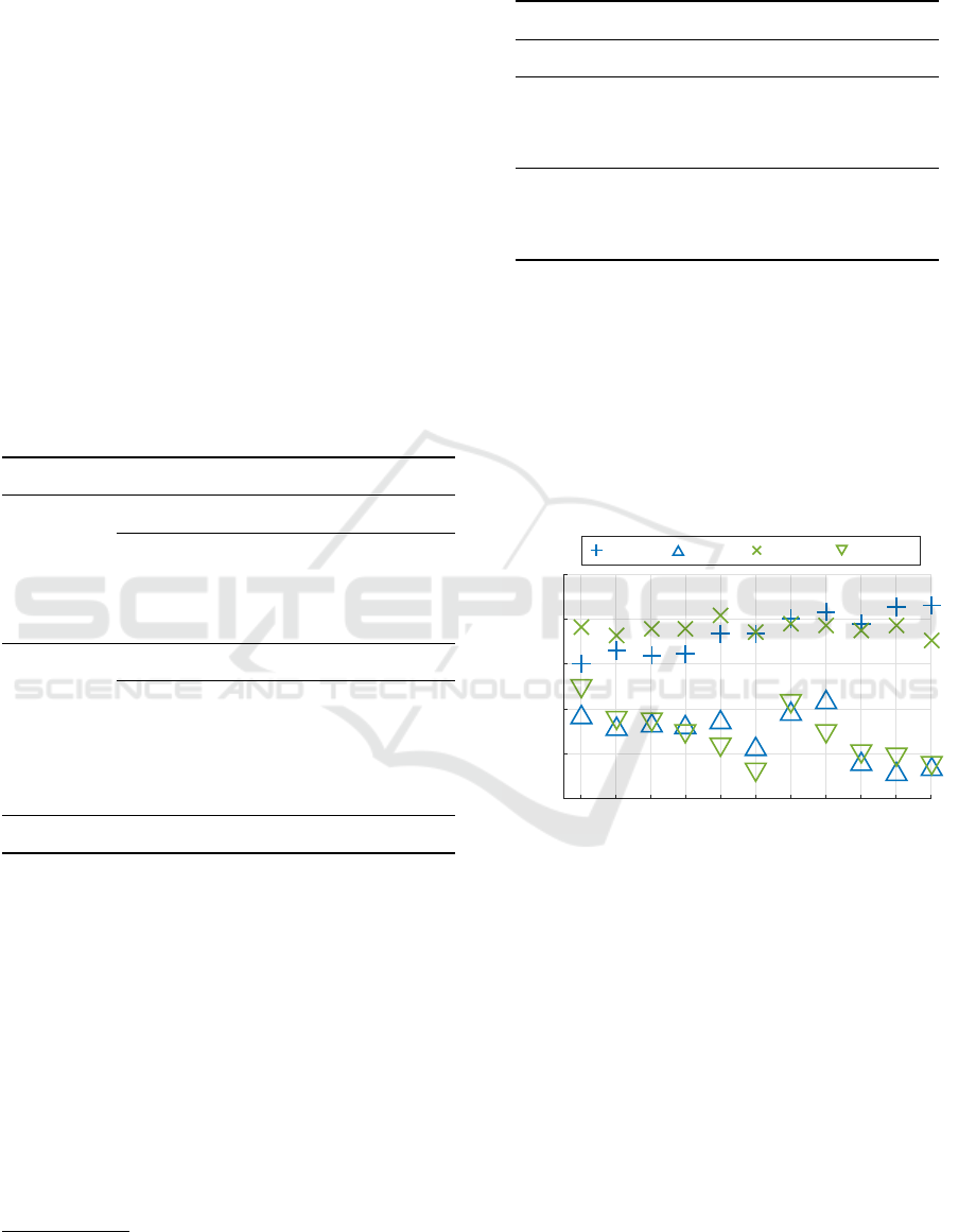
each subset has its own optimum (ﬁgure 4).

10 15 20 25 30 35 40 45 50 55 60

Window size [s]

0.3

0.35

0.4

0.45

0.5

0.55

Accuracy [%]

HR; 75% HR; 0% EDA; 75%

EDA; 0%

Figure 4: Mean accuracy from 10-fold cross-validated

Decision-Tree trained on the heart rate and EDA feature

subsets. Features were extracted on time windows with

length of 10 to 60 s in 5 s steps. For the sake of clarity only

75 % and 0 % overlap are depicted.

Following the objective to set up a short-term pre-

diction of CW, the window size needs to be as short as

possible. On the other hand, we need to keep a min-

imal length in order to obtain reliable features, e.g.

from the heart rate sensor. We found that a 40 s win-

dow resulted in a good predictive performance con-

cerning the heart rate features as well as the EDA fea-

tures (ﬁgure 4). Hence, for further analysis, we chose

a window size of 40 s with an overlap of 75 %. With

this compromise, we ﬁt with the classiﬁcation accura-

cies and keep the window size short at the same time.

Nevertheless, due to the overlap, we obtain a new esti-

Fine-Grained Prediction of Cognitive Workload in a Modern Working Environment by Utilizing Short-Term Physiological Parameters

mate every 10 s. The chosen window length is by 20 s

smaller compared to related work from (Sun et al.,

2012) or (Karthikeyan et al., 2013).

Next, we select an optimal feature subset. From

the ﬁrst test, we found maximum accuracy by using

the full feature set. However, to reduce interdepen-

dencies and redundancies within the full feature set

we want to identify the most valuable features and de-

duce a sparse feature subset. Therefore, we ranked all

features by their information gain (table 3).

Table 3: Average information gain and standard deviation

for the top 12 ranked features. Selected features for the

sparse feature subset are printed bold.

Feature Information Gain

Minimum EDA 0.486 ±0.006

Average SCL 0.451 ±0.004

Average EDA 0.451 ±0.004

Maximum EDA 0.416 ±0.003

Average touch duration 0.361 ±0.004

Average touch pressure 0.333 ±0.003

Minimum heart rate 0.323 ±0.020

Maximum heart rate 0.228 ±0.012

Average heart rate 0.199 ±0.004

standard deviation SCR 0.151 ±0.003

Average RR 0.116 ±0.003

Maximum GSR peak promi-

nence

0.098 ±0.002

Using information gain, we found EDA features

to be most important. Although the touch fea-

tures showed worst predictive performance before-

hand (Decision-Tree, table 2), they were ranked sec-

ond most important after the EDA features. With fur-

ther analysis, we have to assume that this result is due

to spurious relationship within the experimental de-

sign. We must note that the expected count of touch

events was not evenly distributed among the different

phases of the experiment or the demanded CW levels.

Furthermore, there was no control setting for touch

pressure or duration, between the touch intensive and

challenging phases (phase 3 and 5) and those phases

that required only few or no touch inputs (phase 1, 2,

4). For this reason, we withdraw touch features from

further analysis.

To reduce the total complexity of the feature

space, the maximum prominence peak feature (de-

rived from the EDA signal) was also withdrawn. The

resulting sparse feature set contains the 9 most valu-

able features (regarding information gain), which in-

clude 5 features based on EDA and 4 heart rate based

features (table 3).

3.3 Predictive Performance

To evaluate the quality of the selected feature subset,

we tested multiple classiﬁers and compared their ac-

curacy (table 4).

Lowest accuracy resulted from Na

ıve Bayes clas-

siﬁer (45.09 ±2.08 %). We tested normal distribu-

tions as well as multiple kernel smoothing density

estimates for the probability density. Regardless of

the conﬁguration, no perceptibly difference in the ac-

curacy could be found. One explanation for the low

accuracy is the lack of independence concerning the

feature set. However, a thorough investigation of the

cause is not part of this work.

For the Decision-Tree based classiﬁer an average

accuracy of 60.13 ±4.05 % was achieved. In order

to avoid over-ﬁtting, we chose a limit of 100 splits

per tree. Maximum average sensitivity is found on

level 1 (80.49 ±7.56 %). However, the mean sen-

sitivity considering levels 2, 3 and 4 reached only

56.75 ±9.45 %. Thus, the misclassiﬁcations (or in-

accuracy) mainly resulted from the confusions on the

CW levels 2, 3 and 4. Comparable results are found

with the classiﬁer’s speciﬁcity.

The usage of k-Nearest Neighbor resulted in an

enhanced accuracy and overall sensitivity. Again,

the highest sensitivity is found with level 1

(82.14 ±5.35 %). Compared to the Decision-Tree

based classiﬁer, the critical confusion on self-reported

CW levels 2, 3 and 4 is reduced (sensitivity:

65.38 ±6.75 %). However, we noticed a continu-

ous drop of the accuracy with a growing neighbor-

hood. Best results were found with k = 1, which

could suggest an over-ﬁtted model. For instance if

the neighborhood is set to k = 10, accuracy declines

to 58.96 ±2.05 %.

Using Support Vector Machine we were able to

further reduce confusion in the mid-levels (sensiti-

vity: 69.10 ±7.74 %) and therefore increase the over-

all accuracy to 71.00 ±3.36 %. Best results were

archived with radial-basis kernel, although usage of

Gaussian or polynomial kernel did only slightly affect

the predictive performance.

In consideration of the observed confusion in the

mid-levels of the CW prediction, we infer both the

target values (self-reported CW) and the predictors

(EDA, HR) to be noisy. Taking the assumption of

noisy predictors and target values into account, we

chose Gaussian Process Regression as an additional

learner for the comparison. Gaussian Process Regres-

sion is well known to act as a linear smoother and

therefore generally provide good predictive power in

noisy settings (Quadrianto et al., 2010). Indeed, the

Gaussian Process based classiﬁcation outperformed

the other methods with an accuracy of 74.05 % (ﬁg-

BIOSIGNALS 2016 - 9th International Conference on Bio-inspired Systems and Signal Processing

Table 4: Comparison of different classiﬁers based on the sparse feature subset in descending order of 5-class accuracy. All

tests are 10-fold cross validated. Standard deviation during the cross correlation is given with the mean accuracy.

Classiﬁer Normalization Settings Accuracy, 5-class Accuracy, 2-class

Gaussian Process min-max Mat

ern kernel 74.05 ±3.11 % 96.03 ±1.47 %

Support Vector Machine z radial-basis kernel 71.00 ±3.36 % 91.43 ±1.51 %

k-Nearest Neighbor z euclidean distance 67.90 ±3.98 % 92.10 ±2.34 %

Decision-Tree min-max pruned; 100 split limit 60.13 ±4.05 % 90.85 ±1.76 %

ıve Bayes min-max Gaussian kernel 45.09 ±2.08 % 84.37 ±3.20 %

True class

1 2 3 4 5

Predicted class

17.5 %

2.9 %

0.0 %

85.7 %

(14.3 %)

0.8 %

17.1 %

6.7 %

0.4 %

0.0 %

68.3 %

(31.7 %)

0.0 %

3.8 %

21.7 %

2.9 %

0.0 %

76.5 %

(23.5 %)

0.0 %

0.4 %

3.3 %

18.3 %

0.0 %

83.0 %

(17.0 %)

0.0 %

1.7 %

2.5 %

60.0 %

(40.0 %)

95.5 %

(4.5 %)

70.7 %

(29.3 %)

68.4 %

(31.6 %)

78.6 %

(21.4 %)

100.0 %

(0.0 %)

77.1 %

(22.9 %)

Figure 5: Confusion matrix for the best Gaussian Pro-

cess based CW prediction (during 10-fold cross-validation).

Last row contains sensitivity together with false negative

rate (bracketed). The last column contains precision to-

gether with false discovery rate (bracketed).

ure 5). Additionally, the mean sensitivity concern-

ing predicted CW level 2, 3 and 4 was enhanced

(72.95 ±8.10 %).

Still, not all uncertainties are covered by the Gaus-

sian Process. This can easily be seen by shrinking the

classiﬁcation task to a binary problem. In this case

self-reported CW level 1 is interpreted as no CW. All

remaining levels are taken as present CW. By reduc-

ing the machine learning task to this binary problem,

the average accuracy for the Gaussian Process reaches

up to 96.03 ±1.47 %. For the binary classiﬁcation

task, the ranking of the predictive power (accuracy) of

the other tested classiﬁers remains mainly unchanged.

In contrast to the ﬁne-grained tasks, the Na

ıve Bayes

classiﬁer also provided an acceptable classiﬁcation

rate.

4 DISCUSSION

Within this work, we successfully demonstrated a

ﬁne-grained prediction of CW. By focusing on a ﬁne-

grained prediction based on short-term signals, we ex-

tended the complexity of the classiﬁcation task. Ad-

ditionally, we reached the accuracy of today’s state of

the art publications for the binary classiﬁcation task.

In comparison, the ﬁne-grained classiﬁcation resulted

in a lower overall accuracy. This was explained by a

low sensitivity regarding mid-level CW levels. This

observed variation in the self-reported CW levels is

partly explained due to the subjective perception of

CW. In future work the usage of more detailed self-

reports (e.g. based on NASA- Task Load Index (Hart

and Staveland, 1988)) could overcome this issue. Ad-

ditionally, performance measures like error rate or

time-on-task could further clarify the level of sub-

jectively perceived CW. Nevertheless, regarding the

Gaussian Process model, misclassiﬁcation rarely ex-

ceeded more than one class (or level). Therefore, de-

spite the lower overall accuracy, the ﬁne-grained pre-

diction should be favorable, because it facilitates a de-

tailed speciﬁcation of the perceived CW.

Although Gaussian Process showed best accu-

racy, Support Vector Machine yielded comparable

accuracy. As Support Vector Machines are more

widespread and computationally efﬁcient implemen-

tations are commonly available, they might be used

preferentially.

Ranking of the extracted features revealed EDA

features to contain maximum information content, di-

rectly followed by the heart rate features. As empha-

sized by (Sun et al., 2012) care has to be taken if heart

rate is chosen as a predictor, because it is possibly in-

ﬂuenced by means of physical activity. However, dur-

ing our experiment the subjects were monitored by the

experimenter, thus we can exclude physical activity as

confounding factor. Nevertheless, the observed con-

founding inﬂuence of the touch features has to be con-

sidered in future tablet computer based experiments.

Yet, we found that even a narrow short-term fea-

ture subset is sufﬁcient to precisely estimate a per-

Fine-Grained Prediction of Cognitive Workload in a Modern Working Environment by Utilizing Short-Term Physiological Parameters

son’s cognitive workload. This is a mandatory re-

quirement in order to set up an adaptive assistive sys-

tem, which is capable of balancing a given tasks’

complexity accordingly to the users cognitive capac-

ity.

5 SUMMARY AND CONCLUSION

We were able to achieve a ﬁne-grained prediction of

cognitive workload (stress), which exceeds the com-

plexity of the ordinary binary classiﬁcation task. Ad-

ditionally, short-term feature were utilized. To re-

produce a realistic setting, modern working environ-

ments were simulated in the presented experimen-

tal setup. The subjects self-reported their perceived

CW directly after each task. After the preprocessing

we were able to extract a total of 49 features. The

most signiﬁcant features and their ideal window size

and overlap were determined with an initial estimate

based on 10-fold cross-validated Decision-Trees. The

identiﬁed sparse feature subset contains 9 features,

which include 5 features based on EDA and 4 heart

rate based features. The feature subset was then eval-

uated, by comparing the accuracy of multiple well es-

tablished machine learning methods.

In conclusion, we achieved a classiﬁcation accu-

racy of 96.03 % for the binary CW prediction task and

an accuracy of 74.05 % for the ﬁne-grained predictive

model. This is likely to enable the development of

more advanced assistive technology that can precisely

adjust to the user’s requirement in modern working

environments.

In future work we plan to integrate the utilized

sensors into a wearable and hands-free system. This

will allow ﬁeld studies in real working environments

including skilled manual work. Additionally, the us-

age of more detailed self-reports is planned. Further-

more, we want to investigate how our ﬁne-grained

prediction of CW can be used to adapt the complexity

of a task to the user’s needs.

ACKNOWLEDGEMENTS

This research was supported by the DFG CoE 277:

Cognitive Interaction Technology (CITEC), the Ger-

man Federal Ministry of Education and Research

(BMBF) within the Leading-Edge Cluster ”Intelligent

Technical Systems OstWestfalenLippe” (it’s OWL),

managed by the Project Management Agency Karl-

sruhe (PTKA), the BMBF project ALUBAR, and the

PhD program ”Design of Flexible Work Environ-

ments - Human-Centric Use of Cyber-Physical Sys-

tems in Industry 4.0” supported by the North Rhine-

Westphalian funding scheme ”Fortschrittskolleg”.

The authors are responsible for the contents of this

publication.

The authors would like to thank Mindﬁeld for pro-

viding the API for their eSense Skin Response sys-

tem.

REFERENCES

Bishop, C. M. (2006). Pattern Recognition and Machine

Learning (Information Science and Statistics), chapter

Kernel Methods, pages 291–323. Springer New York.

Botthof, A. and Hartmann, E. (2015). Zukunft der Arbeit in

Industrie 4.0 - Neue Perspektiven und offene Fragen.

In Botthof, A. and Hartmann, E. A., editors, Zukunft

der Arbeit in Industrie 4.0, pages 161–163. Springer

Berlin Heidelberg.

Bowling, N. A. and Kirkendall, C. (2012). Workload: A

Review of Causes, Consequences, and Potential Inter-

ventions, pages 221–238. John Wiley & Sons, Ltd.

Cain, B. (2007). A review of the mental workload liter-

ature. In RTO-TR-HFM-121-Part-II. NATO Science

and Technology Organization.

Choi, J., Ahmed, B., and Gutierrez-Osuna, R. (2012). De-

velopment and evaluation of an ambulatory stress

monitor based on wearable sensors. IEEE Trans-

actions on Information Technology in Biomedicine,

16(2):279–286.

Choi, J. and Gutierrez-Osuna, R. (2009). Using heart rate

monitors to detect mental stress. In Sixth International

Workshop on Wearable and Implantable Body Sensor

Networks, pages 219–223.

Dietterich, T. G. and Bakiri, G. (1995). Solving multiclass

learning problems via error-correcting output codes.

Journal of artiﬁcial intelligence research, pages 263–

286.

eSense Skin Response (2015). Biofeedback system. Mind-

ﬁeld Biosystems Ltd., Berlin, Germany.

urnkranz, J. (2010). Decision tree. In Sammut, C. and

Webb, G., editors, Encyclopedia of Machine Learn-

ing, pages 263–267. Springer US.

Harris, W., Hancock, P., and Arthur, E. (1993). The effect of

taskload projection on automation use, performance,

and workload. In Proceedings of the Seventh Interna-

tional Symposium on Aviation Psychology.

Hart, S. G. and Staveland, L. E. (1988). Development of

NASA-TLX (task load index): Results of empirical

and theoretical research. In Human Mental Workload,

volume 52, pages 139–183. North-Holland.

Healey, J. and Picard, R. (2005). Detecting stress during

real-world driving tasks using physiological sensors.

IEEE Transactions on Intelligent Transportation Sys-

tems, 6(2):156–166.

Isshiki, H. and Yamamoto, Y. (1994). Instrument for mon-

itoring arousal level using electrodermal activity. In

BIOSIGNALS 2016 - 9th International Conference on Bio-inspired Systems and Signal Processing

Proceedings of IEEE International Conference on In-

strumentation and Measurement Technology, pages

975–978. IEEE.

Jorna, P. G. (1992). Spectral analysis of heart rate and psy-

chological state: a review of its validity as a workload

index. Biological psychology, 34(2-3):237–257.

Karthikeyan, P., Murugappan, M., and Yaacob, S. (2013).

Detection of human stress using short-term ECG and

HRV signals. Journal of Mechanics in Medicine and

Biology, 13(02):1350038.

Keogh, E. (2010). Nearest neighbor. In Sammut, C. and

Webb, G., editors, Encyclopedia of Machine Learn-

ing, pages 714–715. Springer US.

Malik, M., Bigger, J. T., Camm, A. J., Kleiger, R. E.,

Malliani, A., Moss, A. J., and Schwartz, P. J. (1996).

Heart rate variability. European Heart Journal,

17(3):354–381.

MATLAB (2015). Version 8.5.0 (R2015a). The MathWorks

Inc., Natick, Massachusetts.

MIO Alpha (2013). Heart rate watch. Physical Enterprises

Inc. (Mio Global), Canada, Vancouver.

Nexus 10 (2012). GT-P8110. Google Inc.; Samsung Elec-

tronics.

Polar H6 (2012). Model: X9. Polar Electro Oy, Finland,

Kempele.

Quadrianto, N., Kersting, K., and Xu, Z. (2010). Gaus-

sian process. In Sammut, C. and Webb, G., editors,

Encyclopedia of Machine Learning, pages 428–439.

Springer US.

QuickAmp (2015). Biofeedbacksystem. Brain Products

GmbH, Gilching, Germany.

Rasmussen, C. E. and Nickisch, H. (2010). Gaussian pro-

cesses for machine learning (GPML) toolbox. Journal

of Machine Learning Research, 11:3011–3015.

Rouse, W., Edwards, S., and Hammer, J. M. (1993). Model-

ing the dynamics of mental workload and human per-

formance in complex systems. IEEE Transactions on

Systems, Man, and Cybernetics, 23(6):1662–1671.

Singh, D., Vinod, K., and Saxena, S. (2004). Sampling

frequency of the RR interval time series for spectral

analysis of heart rate variability. Journal of medical

engineering & technology, 28(6):263–272.

Stroop, J. R. (1935). Studies of interference in serial ver-

bal reactions. Journal of Experimental Psychology,

18(6):643–662.

Sun, F.-T., Kuo, C., Cheng, H.-T., Buthpitiya, S., Collins,

P., and Griss, M. (2012). Activity-aware mental stress

detection using physiological sensors. In Gris, M. and

Yang, G., editors, Mobile Computing, Applications,

and Services, volume 76, pages 211–230. Springer

Berlin Heidelberg.

Tarvainen, M., Ranta-aho, P., and Karjalainen, P. (2002).

An advanced detrending method with application to

HRV analysis. IEEE Transactions on Biomedical En-

gineering, 49(2):172–175.

Wallhoff, F., Ablassmeier, M., Bannat, A., Buchta, S.,

Rauschert, A., Rigoll, G., and Wiesbeck, M. (2007).

Adaptive human-machine interfaces in cognitive pro-

duction environments. In Proceedings of IEEE Inter-

national Conference on Multimedia and Expo, pages

2246–2249.

Webb, G. (2010). Na

ıve bayes. In Sammut, C. and Webb,

G., editors, Encyclopedia of Machine Learning, pages

713–714. Springer US.

Wijsman, J., Grundlehner, B., Liu, H., Hermens, H., and

Penders, J. (2011). Towards mental stress detection

using wearable physiological sensors. In Proceedings

of IEEE Engineering in Medicine and Biology Society,

pages 1798–1801.

Witten, I. H. and Frank, E. (2005). Data Mining: Practi-

cal Machine Learning Tools and Techniques. Morgan

Kaufmann Publishers Inc., San Francisco, CA, USA,

second edition.

Young, M. S. and Stanton, N. A. (2002). Attention and au-

tomation: New perspectives on mental underload and

performance. Theoretical Issues in Ergonomics Sci-

ence, 3(2):178–194.

APPENDIX

Table 5: Selected methods used for feature calculation.

categorie function deﬁnition

time mean µ =

∑

i=1

standard

deviation

σ =

n−1

∑

i=1

−µ)

statistical skew

∑

i=1

−µ)

kurtosis

∑

i=1

−µ)

heart rate

variability

NN50

∑

n−1

i=1

−x

i+1

> .05)

RMSSD

∑

i=1

−x

i+1

)

SDSD σ((x

−x

)... (x

n−1

−x

))

SD1

√

.5 ·SDSD

SD2

(2 ·SDSD

) −(.5 ·σ

(x))

SD12

SD1

/SD2

(spectral) VLF energy 0.00 to 0.04 Hz

LF energy 0.04 to 0.15 Hz

HF energy 0.15 to 0.40 Hz

nLF normalized energy (

/LF+HF )

nHF normalized energy (

/LF+HF )

LF/HF

/HF

geometric

(peak)

count number of peaks

prominence distance between to successive

peaks

width distance between the two mini-

mums surrounding a peak

area integral between the two mini-

mums surrounding a peak

Fine-Grained Prediction of Cognitive Workload in a Modern Working Environment by Utilizing Short-Term Physiological Parameters