Interesting Regression- and Model Trees Through Variable Restrictions

Rikard K

onig

, Ulf Johansson

, Ann Lindqvist

and Peter Brattberg

Department of Information Technology, University of Bor

as, SE-501 90, Bor

as, Sweden

Operational data and analysis, REIO, Scania CV AB, SE-151 87, S

odert

alje, Sweden

Keywords:

Predictive Modeling, Model Trees, Interestingness, Regression, Vehicle Modeling, Golf.

Abstract:

The overall purpose of this paper is to suggest a new technique for creating interesting regression- and model

trees. Interesting models are here deﬁned as models that fulﬁll some domain dependent restriction of how

variables can be used in the models. The suggested technique, named ReReM, is an extension of M5 which

can enforce variable constraints while creating regression and model trees. To evaluate ReReM, two case

studies were conducted where the ﬁrst concerned modeling of golf player skill, and the second modeling of

fuel consumption in trucks. Both case studies had variable constraints, deﬁned by domain experts, that should

be fulﬁlled for models to be deemed interesting. When used for modeling golf player skill, ReReM created

regression trees that were slightly less accurate than M5s regression trees. However, the models created with

ReReM were deemed to be interesting by a golf teaching professional while the M5 models were not. In the

second case study, ReReM was evaluated against M5s model trees and a semi-automated approach often used

in the automotive industry. Here, experiments showed that ReReM could achieve a predictive performance

comparable to M5 and clearly better than a semi-automated approach, while fulﬁlling the constraints regarding

interesting models.

1 INTRODUCTION

Freitas (2002) argues that three general properties

should be fulﬁlled by a predictive model; i.e., it

should be accurate, comprehensible, and interesting.

Accuracy is deﬁned by some score function that de-

scribes how well the model solves the predictive prob-

lem. For regression tasks, typical score functions in-

clude mean absolute error (MAE), mean root square

error (RMSE) and the Pearson Correlation (r). Com-

prehensibility is a subjective quality which entails that

the reason behind a prediction must be understand-

able. Factors, such as which and how many functions

are used, the number of parameters the model con-

tains, and even the structure, will affect how a model

is perceived.

The last property, interestingness, is another very

subjective quality which can be hard to achieve. Nor-

mally, simple and rather vague qualities, e.g., that the

discovered knowledge should capture unknown rela-

tionships in the data or fulﬁll some user-deﬁned con-

straints, are used to evaluate whether a model is in-

teresting or not. Freitas (2002) also points out that

even if interestingness obviously is a very important

property, very few techniques are designed to ﬁnd in-

teresting knowledge. Instead accuracy or comprehen-

sibility is normally the focus of studies related to pre-

dictive modeling. This is a problem since the hypoth-

esis that best ﬁt the data is not necessarily the one

that is most interesting. Dietterich (1996) notes that

if an algorithm searches a very large hypothesis space

and outputs a single hypothesis, then in the absence

of huge amounts of training data, the algorithm will

need to make many more or less arbitrary decisions,

decisions which might be different if the training set

were only slightly modiﬁed. This is called informa-

tional instability; i.e., instability caused by the lack of

information. Thus many machine learning techniques

ﬁnd solutions which are precise but not interesting,

according to experts; see e.g., (Grbczewski and Duch,

2002)

When performing data analysis for engineering

applications, it is vital that both models and results

can be explained in terms that make sense for the en-

gineer. If this is not the case, the results from the anal-

ysis are normally not interesting or actionable. Tra-

ditionally, most analysis has been done using tech-

niques and methods from the ﬁeld of statics. Most of-

ten, a hypothesis based on domain knowledge is ver-

iﬁed and reﬁned using statistical tests and methods.

König, R., Johansson, U., Lindqvist, A. and Brattberg, P..

Interesting Regression- and Model Trees Through Variable Restrictions.

In Proceedings of the 7th International Joint Conference on Knowledge Discovery, Knowledge Engineering and Knowledge Management (IC3K 2015) - Volume 1: KDIR, pages 281-292

ISBN: 978-989-758-158-8

281

Since the hypotheses are based mainly on engineer-

ing domain knowledge, they immediately make sense

to the engineers. At the same time, these methods

are restricted to the imagination of the engineer, since

they rely on his or her knowledge.

The purpose of this paper is to demonstrate

a straightforward technique for creating interesting

regression- and model trees by including user con-

straints related to how variables may be used. The

main idea is to combine a data driven approach and

the typical engineering approach where predeﬁned

hypotheses are tested and reﬁned. More speciﬁcally,

Quinlan (1992)s M5 algorithm is extended to enforce

problem constraints when building regression- and

model trees. A positive side effect is that the search

space is reduced, which should increase the possibil-

ity of ﬁnding an both accurate an interesting model.

The usefulness and generality of the suggested tech-

nique is demonstrated in two very different real-world

case studies, modeling of golf player skill and model-

ing of driver inﬂuence on fuel consumption of trucks.

2 RELATED WORK

Decision trees are arguably the most popular pre-

dictive technique producing comprehensible models.

Furthermore, for regression problems, which is the fo-

cus of this study, the M5 algorithm, ﬁrst presented in

Quinlan (1992), is one of the most powerful and ﬂex-

ible. Since M5 is also the basis for the new technique

suggested in this study, it is presented in more detail

below. The following subsection then presents related

work regarding the creation of interesting predictive

models.

2.1 Decision Trees

Quinlans M5, ﬁrst presented in (Quinlan, 1992), is a

decision tree inducer used to create comprehensible

models in the form of regression trees or model trees.

Regression trees are trees with numeric constant in

the leaves, while model trees use linear regression.

Regression trees are easy to generate and interpret,

but normally not very accurate. Hence, Quinlan sug-

gested the use of model trees. M5 model trees is a a

piecewise linear regression, created by selecting each

split in a way that minimizes the standard deviation of

the subtrees. When the tree is fully grown, linear re-

gressions are created using standard regression tech-

niques for each node in the tree. Next, each model is

simpliﬁed by considering the estimated error at each

node. If a model consisting of a subset of the param-

eters used in the original model has a lower estimated

error according to equation 1, (where n is the num-

ber of instances reaching that leaf and v is the number

of parameters of the model), it replaces the original

model.

e = e ∗ (n + v)/(n − v) (1)

Finally, each non-terminal node is compared to its

subtrees in the same way. If the estimated error of

the node is lower than its subtree, the subtree is re-

placed by the model. Model trees are in general

both more accurate and more compact than regres-

sion trees. Another notable difference is that model

trees can extrapolate outside the range of the train-

ing instances. Nevertheless, regression trees are also

supported in M5, since they are in general deemed to

be more comprehensible. When creating regression

trees a single constant, i.e., the average value of all

training instances reaching a leaf, is chosen instead of

a linear regression. Even if a regression trees often

need many leaves to be accurate, and hence may look

complex, they are most often only complex when the

whole tree is considered. However, for a single leaf

only the splits leading to that leaf need to be consid-

ered. Since the number of leaves grows exponentially,

with the depth of a the tree the number of splits that

must be checked are normally quite manageable.

2.1.1 Creating Interesting Models

One basic assumption regarding interesting trees is

that they must be accurate enough while still being

comprehensible. Hence, much work has been focused

on creating constrained decision trees, i.e., trees that

are constrained according to some criterion, most of-

ten accuracy or complexity. Garofalakis et al. (2003)

for example, proposes a technique where the user may

specify either a minimum accuracy or a maximum

complexity while optimizing the other criteria, e.g. if

a maximum complexity is set, the tree with the high-

est accuracy with sufﬁciently low complexity is re-

turned. In this way, it is ensured that the trees are

both easy to understand and have a good accuracy.

The same approach is taken by Struyf and Dzeroski

(2006) with the difference that a large tree is ﬁrst built,

before it is pruned until it fulﬁls the complexity con-

straint set by the user. Nijssen and Fromont (2010)

explores a technique for constraining trees using item

set lattices. Here, decision trees are again constrained

with regards to accuracy and complexity, but other

constraints related to the creation of the tree are also

explored, e.g., minimum number of samples in a leaf,

classiﬁcation cost, and enforcing a signiﬁcant major-

ity in the leaves.

When interestingness of trees are evaluated, corre-

lation with existing domain knowledge or constraints

KDIR 2015 - 7th International Conference on Knowledge Discovery and Information Retrieval

282

are often evaluated. Hence, to create more interesting

models, many techniques include knowledge in the

form of costs, thus becoming cost-sensitive to errors

or the acquiring of a variable value. 50 such algo-

rithms are described in (Lomax and Vadera, 2013).

Another approach is to use some knowledge about

the importance of a variable when used for prediction,

and include it in training of the model, see e.g., (Iqbal

et al., 2012) for a decision tree technique or (Iqbal,

2011) for a neural network technique. Yet another ap-

proach, presented in (N

nez, 1991) uses information

about hierarchies related to the attributes in combi-

nation with attribute cost to reduce the classiﬁcation

costs and increase the generalization of the produced

decision trees.

What all these techniques have in common is that

they report enhanced results when domain knowledge

is somehow incorporated in predictive models. This

is of course an encouraging but expected result, since

domain knowledge, in whatever form, typically adds

valuable information not present in the data. An-

other thing these techniques have in common is that

they are in general advanced in the form of domain

knowledge they work with, e.g., feature importance,

attribute hierarchies or attribute costs. In many cases

this type of information does not exist but there is

still some kind of simple domain knowledge, like re-

striction of the relation between variables, that can be

used. Hence, we argue for a more straightforward ap-

proach for these situations.

None of the techniques for creating constrained

decision trees or for including domain knowledge

mentioned above, fulﬁll the criteria set for interest-

ing trees in this study. Hence, this paper does not aim

to make a quantitative comparison against these tech-

nique but to suggest and demonstrate the usefulness

of the novel technique, presented in 4.1. However,

some kind of benchmark is of course needed, so the

proposed technique is evaluated against a straightfor-

ward approach based on standard decision trees.

3 BACKGROUND

The following sections describe the two problem do-

mains, i.e., creating interesting models for predicting

golf player skill and the driver’s inﬂuence on fuel con-

sumption in trucks.

3.1 Modeling Golf Player Skill

The ﬁrst case study in this paper explores the possi-

bility to create interesting predictive models of golf

swings. The idea is to help players determine which

aspect of their swing they need to improve. For a pre-

dictive model to be interesting in this scenario it must

be comprehensible and actionable for the player or

at least for a teaching professional. It would for ex-

ample not be very helpful to tell a golfer that he hits

the ball with too much hook or slice (curving the ball

to the left or to the right) and that he should hit the

ball straighter. An interesting model should instead

mainly be expressed in terms of characteristics of the

swing itself.

Golf has a handicap system which is intended to

let players of different skill levels play against each

other on equal terms. Hence, a golfer’s handicap

(Hcp) is an estimation of the player’s skill. The way

a handicap is calculated differs slightly between USA

and Europe, but simply put it is the number of strokes

a player may deduct from his total number of strokes

after 18 holes. If a player ﬁnishes a round with less

strokes than what is intended for his Hcp, the Hcp is

lowered a fraction and if the score is higher the Hcp

is increased. Hence, Hcp is a measure of the over-

all skill of a player, i.e. including putting, short-game

and the long-game.

Since the golf swing itself consists of a very com-

plex chain of movements and the club head moves at

great speeds, it is very hard to evaluate a golf swing

just by manual observation. Naturally many previous

studies have been conducted with the aim of analysing

the swing quantitatively using high speed video, e.g.,

see (Fradkin et al., 2004) or (Sweeney et al., 2013).

Due to tedious manual labor related to video analysis,

these and similar studies only use a relatively small

number of players.

However, lately new technology like the Track-

Man Launch Monitor Radar (TM) (Trackman, 2015)

has made it possible to measure numerous character-

istics of golf swings quantitatively. TM units use a

Doppler radar to register information about the club

head at the point of impact (POI) and the trajectory of

the ball. In total TM returns 27 metrics, described in

section 3.1.1, where seven are related to the club head

and 20 related to the ball ﬂight.

In (Betzler et al., 2012) 10 shots from each of

285 players were recorded using TM and ﬁve 1000Hz

high speed cameras. Here, the aim was to evaluate

the variability in club head presentation at impact and

the resulting ball impact location on the club face,

for a range of golfers with different Hcp. Statistical

test showed that overall, players with lower Hcp, i.e.,

players with Hcp <= 11.4, exhibited signiﬁcant less

variation in all of the evaluated variables. This study

and the other two using high speed cameras, men-

tioned above, have been restricted to analysis of single

variables independently using statistical techniques.

Interesting Regression- and Model Trees Through Variable Restrictions

283

An alternative approach, explored in this study, is

to gather swing data from a large set of golfers and

then model their skill, using regression trees, based

on that data. If the model is sufﬁciently accurate

and comprehensible, it could then be used to explain

the difference in skill based on swing characteristics.

More technically, we try to model golf player skill us-

ing data collected with a TM unit, using player handi-

caps as the target. An interesting model is here de-

ﬁned as a model that explains the skill of a player

based mainly on swing related variables.

3.1.1 Data

In this study a total 277 golf players with Hcp ranging

from +4 to 36, with an average Hcp of 12.8, were

recorded using TM.

To collect data from a player the radar was posi-

tioned three meters behind and slightly to right of the

player. Next, the radar was aimed (using the Track-

man Performance Studio software) at a ﬂag approxi-

mately 250m away. Before recording a player he was

ﬁrst allowed to hit some warm up shots. Next, ﬁve

consecutive strokes was recorded using the player’s

own 7-iron. The players were told to hit the balls in

the direction of the ﬂag using a normal full stroke,

but disregarding any wind present. The wind was in-

stead handled by using TM’s built in normalization

functionality. When normalizing ball data, TrackMan

utilizes information from the club head at impact to

correct deviations caused not only by the wind, but

also from temperature, altitude and ball type. The TM

metrics recorded used in this study are presented be-

low. For more detailed explanations see (Trackman,

2015):

The variables related to the club head are:

• ClubSpeed - Speed of the club head instant prior

to impact.

• AttackAngle - Vertical movement of the club

through impact.

• ClubPath - Horizontal movement of the club

through impact.

• SwingPlane - Bottom half of the swing plane rel-

ative to ground.

• SwingDirection - Bottom half of the swing plane

relative to target line.

• DynLoft - Orientation of club face, relative to the

plumb line, at POI.

• FaceAngle - Orientation of club face, relative to

target line, at POI.

• FaceToPath - Orientation of club face, relative to

club path, at POI. (+) = open path, (-) = closed

path.

The variables related to the ball ﬂight are:

• BallSpeed,BallSpeedC - Ball speed instant after

impact, speed at landing.

• SmashFactor - Ball speed / club head speed at in-

stant after POI.

• LaunchAngle - Launch angle, relative horizon,

immediately after impact.

• LaunchDirection - Starting direction, relative to

target line, of ball immediately after impact. (+) =

right, (-) = left.

• SpinRate - Ball rotation per minute instant after

impact.

• SpinAxis - Tilt of spin axis. (+) = fade / slice, (-)

= draw / hook.

• VertAngleC - Ball landing angle, relative to

ground at zero elevation.

• Height, DistHeight, SideHeight - Maximum

height of shot at apex, distance to apex, apex dis-

tance from target line.

• LengthC, LengthT - Length of shot, C = calcu-

lated carry at zero elevation, T = calculated total

including bounce and roll at zero elevation.

• SideC, SideT - Distance from target line, C = at

landing, T = calculated total including bounce and

roll. (+) = right, (-) = left.

To get one comprehensive value for each met-

ric, the median stroke (based on LengthC), was used.

Median values are preferred, as argued by (Broadie,

2008), since they disregard potentially really poor

shots which otherwise could lead to misleading aver-

ages. Furthermore, using a single swing also ensures

that all recorded values relate to each other.

Since previous work like (Betzler et al., 2012) has

shown that better players are more consistent, stan-

dard deviations (based on all 5 strokes) of each of the

27 metrics were also calculated and included as vari-

ables.

An important issue is how to best represent each

metric for predictive modeling techniques. Most met-

rics, like Carry Length, has a straightforward repre-

sentation, but metrics related to angles need some ex-

tra consideration. Face Angle is one example where

the chosen representation is very important, since the

angle can be both positive and negative, i.e. represent-

ing the face pointing to the right or left of the target

line. If no transformation is used, a big negative angle

would be considered as smaller than a small positive

angle. However, in relation to the target line, which is

more relevant for the quality of a swing, the opposite

is true. Hence, metrics related to the target line were

replaced with two new variables where the ﬁrst was

the absolute values and the second was a binary vari-

able representing if the original angle was positive or

not. Metrics related to vertical angles, i.e., Attack An-

KDIR 2015 - 7th International Conference on Knowledge Discovery and Information Retrieval

284

gle, Launch Angle, were not modiﬁed. Finally, since

Hcp is designed to be an estimation of a player’s skill

it was selected as the dependent variable.

3.2 Modeling Fuel Consumption

The second case study models fuel consumption in

trucks manufactured by Scania. A unique modular

system is one of the most important success factors

for Scania. Modularization means that the interfaces

between component series are standardized to ensure

that they ﬁt together in many different combinations.

The overall purpose of the modular system is to en-

sure that customers get a highly optimized product,

still built from standardized parts, thus offering cus-

tomers tailor-made vehicles, while lowering produc-

tion costs for Scania. This highly ﬂexible system, on

the other hand, implies that almost every vehicle is

unique in its combination of different modules. In

fact, it is often said that Scania has an average pro-

duction series of 1.2 similar trucks. Obviously, this is

a great challenge when developing methods for anal-

ysis of operational and diagnostic vehicle data. Fur-

thermore, heavy commercial vehicles also have very

diversiﬁed transport assignments, compared to cars

used for private transportation. The transport assign-

ments of Scania trucks range from light operations

such as the distribution of ﬂowers in the Netherlands,

to heavy operations like transporting 100 ton of stone

from mines on muddy jungle tracks in Africa. Natu-

rally, such diversiﬁed usage further complicates oper-

ational analysis.

In many scenarios, like when modeling the drivers

inﬂuence on fuel consumption, the way variables are

combined is very important for how interesting a

model becomes. First, variables related to the driver

must be included in the model. However due to the

very heterogeneous vehicle ﬂeet neither the conﬁg-

uration of the trucks nor the transport assignment

can be disregarded. Obviously, different types of

trucks have different fuel consumption patterns and

driver actions that is normal for the speciﬁc task,

e.g., while making many stops and idling in heavy

city trafﬁc may be normal behavior, it would be very

strange when performing long haulage with heavy

loads. Hence, an interesting model should be able to

discern the drivers effect on fuel consumption from

the conﬁguration and assignment. A pure data driven

approach would most likely result in a model con-

sisting of a jumble of assignment, conﬁguration and

driver related variables, thus hampering the compre-

hensibility and making analysis extremely cumber-

some, or even impossible.

One frequently applied straightforward approach

to this problem, and for increasing accuracy, is to

manually divide the ﬂeet into subsets of more simi-

lar vehicles, based on for example their transport as-

signments. Next, a variable selection is performed

for each subset which is then modeled using some

multiple linear regression based technique. The main

idea behind this semi-automatic approach, hence-

forth called subset modeling, is that similar instances

should, at least in theory, require fewer regressors and

be modeled more easily, thus resulting in more com-

prehensible and more accurate models. Subset mod-

eling is normally based on domain knowledge, conse-

quently requiring a substantial amount of manual la-

bor if more than a few subsets are to be formed. Still,

it is not sure that the groups formed by the engineers

using their domain knowledge, is the best basis for the

following analysis.

3.2.1 Data

The vehicles that Scania produces contain advanced

networks of different embedded computers called

Electronic Control Units (ECU:s). Data is aggre-

gated over the entire lifetime of an ECU and is up-

loaded to Scania during workshop visits and stored

in a database. The operational data is then combined

with information about the modular system and other

data sources in a data warehouse.

The data set used in the experiments include data

from 33196 vehicles consisting of 43 variables based

on the second to last and the last readouts. The depen-

dent variable was the average fuel consumption be-

tween these readouts and the 43 independent variables

(a small subset of what was available) were calculated

in a similar manner. Only a few of the actual variables

are presented with real names, due to company policy,

but they can however be divided into three subgroups:

Conﬁguration. Variables related to the conﬁguration

of the truck, e.g., number of axles, engine size,

height, length etc.

Assignment. Variables related to the transport as-

signment, e.g. cargo weight, number of stops, dis-

tance, average inclination etc.

Driver. Variables inﬂuenced by the driver, e.g., aver-

age speed, braking, use of cruise control, idling

etc.

More speciﬁcally the data set consisted of:

The aim of this case study is to create a better de-

cision support for truck driver coaching. To do this

the engineers at Scania wanted to be able to explain

the fuel consumption of a truck based on the drivers

actions and the transport assignment. However, since

the conﬁguration of a truck is highly correlated with

Interesting Regression- and Model Trees Through Variable Restrictions

285

Table 1: Characteristics of the dataset.

Property Amount Categorical Continuous

Instances 33196 - -

Variables 43 8 35

Conﬁguration 12 8 4

Assignment 7 7

Driver 24 24

the fuel consumption, the conﬁguration cannot be dis-

regarded. To be actionable and therefore interesting

to Scania, the engineers argued that trucks should be

grouped into subsets using conﬁguration and assign-

ment related variables while the modeling of the fuel

consumption for each subset should be done based on

driver and assignment related variables.

4 METHOD

As described above, the use of subsets modeling is

a well-known and accepted approach in the automo-

tive industry. However, since this division is done

manually and solely based on domain knowledge and

basic statistics, there may be room for improvement.

What appears to be a natural grouping of vehicles for

a domain expert may be far from optimal for predic-

tive modeling. Speciﬁcally, if the grouping is done

based on domain knowledge, it is typically restricted

in complexity, and even to variables that the particu-

lar domain expert has a solid understanding of. At the

same time, a purely data driven approach is not neces-

sary better, since it may well produce none-actionable

models. Hence, we suggest an addition to the M5 al-

gorithm which allow the user to add restrictions for

how the splitting attributes are selected when creat-

ing regression or model trees. The extended algo-

rithm which, to the best of our knowledge, constitute

a straightforward yet novel addition to M5, is hence-

forth called ReReM, i.e., Restricted Regression- and

Model trees.

4.1 ReReM

ReReM was implemented as a modiﬁcation of the

Weka (Blake and Merz, 1998), version of M5, called

M5P. In the standard implementation of M5P, splits

are selected using a standard search for the best split

among all available variables. The suggested exten-

sion modiﬁes this process by restricting the attributes

to be considered. More precisely, only attributes al-

lowed at the current level of the tree are considered

when optimizing the split. The allowed attributes are

speciﬁed by the decision maker and given as a list of

(depth lists), where each depth list contains the al-

lowed variables for a speciﬁc depth. More speciﬁ-

cally the M5P code in WEKA was extended with the

method getVariables (listed below) which was then

called every time a set of variables was requested.

Variables that are to be allowed in the linear regres-

sion leaves of a model tree can also be speciﬁed in

the same way. ReReM can be downloaded from

sites.google.com/site/GetReRem.

public DepthList getVariables(int nodeDepth,

DepthList[] lists){

for(DepthList dl:lists)

if(nodeDepth <= dl.getDepthLimit())

return dl.getAllowedVariables();}

5 EXPERIMENTS

The experiments aim to evaluate the beneﬁts of using

ReReM instead of traditional modeling approaches.

Hence the two case studies are setup according to the

same scheme. First, the purely data driven approach

of using all available data is evaluated. Secondly,

the semi-manual approaches of creating more inter-

esting models using subsets of the original variables

are evaluated. These are the typical approaches that

could be used without ReReM. Finally ReReM are

used with constraints set by domain experts. To in-

crease readability of the experiments the purely data

driven experiments using all data are preceded with

a D, semi-manual experiments with an S and ReReM

experiments with an R.

The experiments related to modeling golf

player skill are evaluated using leave-one-out cross-

validation due to the relatively small number of

records. For experiments related to modeling of fuel

consumption, standard 10-fold cross-validation is

instead used. The predictive performance is reported

using the coefﬁcient of determination (r

) and the

mean absolute error (MAE) when modeling golf

player skill. For the experiments concerning model-

ing of fuel consumption the relative mean absolute

error (RMAE) is reported instead of MAE due to

company policy. RMAE is relative to predicting

the mean value of each training set, e.g. RMAE is

calculated by dividing the MAE of the technique with

the MAE of predicting the mean value.

5.1 Results Modeling Golf Player Skill

In the ﬁrst case study the idea is to help players ﬁg-

uring out what aspect of their swing they need to im-

prove. Hence, the models should be based on parame-

KDIR 2015 - 7th International Conference on Knowledge Discovery and Information Retrieval

286

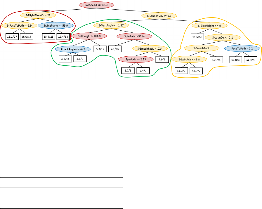
Figure 1: Regression tree based on all data (Exp. D).

ters related to the club rather than the ball ﬂight. Fur-

thermore, since the ﬁrst splits in a decision tree are

more important it is vital that these splits are based

on club related variables. If, instead, the ﬁrst split

was based on, for instance, S-SpinAxis, this would

provide very little information to the player, typically

instead requiring further analysis to determine the

cause. Table 2 presents the results for all experiments

in this case study. These results and the details of the

experiments are discussed in the subsequent sections.

Table 2: Results modeling golf player skill.

Exp SplitV r

MAE Rules

D Club, Ball, STD .415 4.40 17

S Club .244 5.74 6

R Club to depth 3 then All .324 5.37 16

5.1.1 Data Driven Approach

Figure 1 above shows a tree created using the tra-

ditional data driven approach based on all available

data, i.e., club head, ball ﬂight and the standard devi-

ations of all variables. Even if this approach was the

most accurate, (see results for D in table 2), the in-

terestingness of the tree is questionable, at best. Only

three, (marked in green) of sixteen splits are based on

club data, and the more important splits, near the root

of the tree, is based on ball speed and the standard

deviation of ﬂight time and launch direction. Obvi-

ously, instructions based on this tree would require

further analysis of the cause of the standard devia-

tions. Disregarding this, some interesting observa-

tions may still be made. First, the tree groups players

of similar skill in leaves close to each other. There are

four different super groups marked in different col-

ors with the least skilled golfers marked in red and

the most skilled in green. It is also interesting that

the better of the least skilled players, i.e., players with

a predicted Hcp of 15.4, have a ﬂatter swing plane

than the rest. Another interesting observation is that

the best players (marked in green) hit more down on

the ball in the swing, i.e., have a more negative attack

angle. A problem with these observations is, how-

ever, that the they are not applicable without ﬁrst di-

viding the players using ball ﬂight data and standard

deviations, thus severely limiting the usefulness of the

model. Nonetheless, if predictive performance is the

only concern this approach is clearly superior in terms

of r

and MAE.

5.1.2 Semi-automated Approach

The most simple approach of ensuring that the mod-

els are based on club related variables is of course to

create an attribute subsets only containing these vari-

ables. The results of this experiment, i.e., experiment

S is presented in table 2. However, even if some in-

teresting observations could be done, the tree created

with this approach had a substantially worse predic-

tive performance, compared to the purely data driven

approach. More speciﬁcally, the MAE was 5.74 and

0.244 compared to 4.40 and 0.415.

5.1.3 Restricted Approach using ReReM

Since the ﬁrst level of splits are more important for

the interestingness of the models in this case study,

ReReM was setup to enforce restrictions accordingly.

More speciﬁcally, splits at the ﬁrst three levels of the

tree were restricted to club related variables while

the succeeding splits could use all available vari-

ables. The motivation for this was to ﬁnd a compro-

mise between the data driven approach and the semi-

automated approach presented above. Since the mod-

els in experiment D had an average of 4.5 splits in

each branch, a restriction for the ﬁrst three levels was

deemed appropriate to ensure that a sufﬁcient num-

ber of nodes were based on club variables, while still

leaving room for the inclusion of a few other vari-

ables. When comparing the accuracy of ReReM with

Interesting Regression- and Model Trees Through Variable Restrictions

287

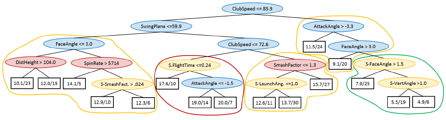
Figure 2: ReReM regression tree where splits to depth 3 are restricted to club data (Exp. R).

the simple approach of using only club data, ReReM

is clearly superior. More speciﬁcally, the tree created

using only club data had a r

of .244 compared to .324

of the ReReM tree and a MAE of 5.37 compared to

5.74. The tree created using all data, i.e., experiment

D, had a r

of .415 but was, for the reasons discussed

in section 5.1.1, deemed to be less interesting. Finally

it is of course interesting to interpret the resulting tree

presented in Figure 2. Again larger super groups of

players at different levels are present. Here, how-

ever, the larger groups are created using splits based

on club data which makes the rules much more inter-

esting. Some observations that can be made are:

• To become a really good player you must be able

to hit the ball with a club speed higher than 85.9.

• The swing plane is again important for differenti-

ating between players of average skill. Here, play-

ers with lower swing planes tend to have a lower

Hcp.

• Among hard hitting players, the players with

higher handicap should hit more down on the ball.

• If a hard hitting player achieves a sufﬁcient attack

angle, the next important feature is the face angle,

i.e., that the face angle should not be too high. A

high face angle results in a launch direction fur-

ther from the target line, which must be counter-

acted by a curved shot which is harder to control.

All of these observations concur with modern swing

theory, except for the importance of the swing plane,

which is a non-trivial ﬁnding, which would be inter-

esting to study further. There are several other in-

teresting rules that can be found in this tree, but the

main point is that the most important splits are based

on club related variables. Hence, it would be simple

to directly suggest a particular exercise to improve the

attack angle, face angle or swing plane. In lower parts

of the tree, ball ﬂight parameters still occur, but only

to discern among similarly skilled golfers. In these

cases, a teaching professional could add valuable in-

formation on what, for example, a player should do to

improve his smash factor. It should also be noted that

the data set consists of a relatively small number of

players and it is possible that a larger data set could

improve the possibility of explaining the difference

based on only club variables.

5.2 Results Modeling Fuel Consumption

ReReM is, simply put, a technique for simplifying

the semi-automatic procedure to subset modeling dis-

cussed in section 3.2, but it may also increase the ac-

curacy by performing a data driven creation of the

subsets. The main idea is to facilitate the use of more

explanatory variables while retaining some control

over how they are used to ensure that the created mod-

els become interesting and actionable. To enable an

comparison with the techniques used in practice, the

experiments of this case study are done using model

trees.

The results of the different approaches are all pre-

sented together in Table 3 to simplify a comparison of

their predictive performance. However, in the analy-

sis, each approach is discussed separately in the sub-

sequent sections. In Table 3, D1 is the purely data

driven approach, S1 and S2 are two different semi-

automated approaches while R1 and R2 use ReReM

to enforce variable restrictions. SplitV and RegrV

are the variables types used in the splits of the de-

cision tree and as regressors, i.e. C=conﬁguration,

A=assignment and D=driver. In experiment S2 and

R1 only two variables, w=weight and s=speed, are al-

lowed for splitting the data. The superscripted letter

signiﬁes if the splits were selected manually (m) or

data driven (d). All experiments are discussed in more

details in the following subsections.

5.2.1 Data Driven Approach

In the ﬁrst experiment, D1, all available data is used

to create a single model tree using M5P. The results

show that the model tree obtained a rather high r

KDIR 2015 - 7th International Conference on Knowledge Discovery and Information Retrieval

288

Table 3: Results for ReReM model trees.

Exp SplitV RegrV r

RMAE #Regr. #Vars.

D1 C,A,D C,A,D .886 .313 33.7 75

S1 - A,D .837 .392 1.0 25

S2 w

A,D .860 .360 9.0 19.9

R1 w

A,D .871 .342 14.2 22.2

R2 C,A A,D .897 .295 32.5 19.7

.886 and a low RMAE of 31.3%. The results are bet-

ter than all other approaches except R2, which will

be discussed later in subsection 5.2.3. The average

size of the model trees produced with this approach is

fairly large with 33.7 regression leaves, where each

regression expression is based on 75 variables. In

a balanced model tree with 33.7 leaves, the average

number of splits needed to reach a leaf is, however,

only slightly higher than 5, i.e., understanding and an-

alyzing the reasons for a speciﬁc prediction is clearly

manageable.

The regression expressions containing 75 vari-

ables, on the other hand, are very hard to analyze

manually. The reason for the large number of vari-

ables is the fact that M5P creates binary variables for

each category of a categorical variable, and also tend

to use most of these resulting binary variables. An-

other problem with model trees created using this ap-

proach is that the different variable types, i.e. conﬁgu-

ration, assignment and driver, are mixed, which is not

very usable in practice. Figure 3 illustrates this prob-

lem by showing a tiny sample tree created with the

same settings as for D1, with the exception of forcing

a higher number of instances per node to produce a

more compact tree. This model tree consists of two

driver related variables (marked in red), one conﬁg-

uration variable (marked in blue) and three variables

related to the conﬁguration, (marked in yellow). The

two driver related variables DriveTime and Braking

cannot be described in more detail here, due to com-

pany policy. The three conﬁguration related variables

are the number of axles of the truck, the horsepower

and var22 which is a conﬁguration related variable

that we are not allowed to describe further, again due

to company policy. Finally, the only assignment spe-

ciﬁc variable present in the tree is weight, i.e., the total

weight including cargo of the truck averaged over the

traveled distance. Naturally, when performing pre-

diction, an instance meeting a split condition is sent

to the left child node of the split and if not to the

right child node. The leaves consist of a reference to

a linear regression, followed by the fuel consumption

relative to the mean and the percentage of the trucks

that reach the leaf. Hence, the leaf farthest to the left

in Figure 3, refers to the linear regression L1, makes

prediction for 4,4% of the trucks, which on average

have a fuel consumption 2% lower than the average

fuel consumption of all trucks. Note that the average

fuel consumption is only presented to facilitate a com-

prehensive interpretation of the trees since the linear

regression cannot be disclosed due to company policy.

The tree in Figure 3 is relatively straightforward

to interpret, i.e., higher values for weight, horsepower,

axles and braking do all result in higher fuel consump-

tion, which is as expected. The ﬁrst split, DriveTime,

is however problematic, for the interpretation of the

tree, since it will result in that driver with similar

trucks and assignments can be modeled using differ-

ent regressions. Another problem was that all regres-

sion expressions included all types of variables. This

was deemed to be unsatisfactory by domain experts,

since they argued that it would be more logical to only

use the more constant conﬁguration related variables

in the decision tree for creating the subsets. For these

reasons, the interestingness of the model was deemed

unsatisfactory in spite of the high predictive perfor-

mance.

5.2.2 Semi-automated Approaches

Due to the reasons mention in section 5.2.1, purely

data driven approaches are rarely used in practice.

Instead some kind of semi-automated approach is

used. Here, two approaches are evaluated in the

experiments S1 and S2. The predictive performances

of these experiments are presented in table 3.

Simple Approach

In the ﬁrst Experiment, S1, the most simple and naive

approach to ensuring that driver related variables are

only present in the regressions, i.e. to not build model

trees but a single multiple linear regression based

on only driver- and assignment related variables, is

evaluated. The results presented in Table 3, does

however show that the models created with this ap-

proach has the worst predictive performance, for both

and RMAE, of all evaluated approaches. Hence,

there is an obvious trade-off between accuracy and

comprehensibility.

Manual Subset Modeling

The second semi-automated approach S2 is the tradi-

tional subset modeling approach discussed in section

3.2. Since the usage of a truck naturally has a huge

impact on its performance, domain experts in this case

recommended nine subgroups based on the average

total weight and average speed of the truck. Each vari-

able was used to split the vehicles into groups with

low (L) medium (M) or high (H) values resulting in

nine subgroups. Table 4 shows the resulting number

of instances in each group.

Interesting Regression- and Model Trees Through Variable Restrictions

289

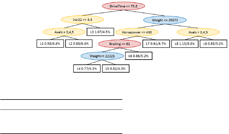
Figure 3: Model tree created using all available variables in both splits and regression (Exp. D1).

Table 4: Vehicles per subset.

L-Weight M-Weight H-Weight

H-Speed 1785 9762 4208

M-Speed 2982 6767 3937

L-Speed 1805 1179 771

When creating linear regressions for the subsets,

only assignment and driver related variables were

considered. Furthermore, to improve the generality

of the regressions a variable selection (shrinking) was

used for each subset using backward elimination. The

conventional 5% signiﬁcation was used as the limit

for the variables to be excluded from the model. Fi-

nally one linear regression was created for each sub-

group. The nine resulting regression expressions were

considered to be the ﬁnal model and were used for the

evaluation.

It is clear from the result in Table 3 that the man-

ual subsets modeling approach was successful since

it improved the performance compared to the simple

approach, using all of the presented measures. The in-

creased accuracy, however, was produced by a more

complex model, i.e., using nine regression models in-

stead of just one. It must be noted, though, that for

a speciﬁc vehicle only one regression needs to be in-

terpreted and the ones created for the subsets were

less complex, containing on average 20 variables. Fi-

nally, even if the manual subset method outperformed

the simple approach, it is still less accurate than the

purely data driven.

5.2.3 Restricted Modeling using ReReM

The manual subset modelling approach, used in

experiment S2, may be suboptimal in mainly two

ways; ﬁrst the subsets created from the selected

variables may be suboptimal and second the variables

chosen may not be the most appropriate ones. To

shed some light on these questions, two experiments

are performed using ReReM. To evaluate how good

the manual subset modeling approach is in ﬁnding

good subsets, a data driven variant of experiment

S2 is ﬁrst evaluated in experiment R1. Second,

experiment R2 evaluates if there are better variables

to base the splits on. It should be noted that these

experiments are only possible due to ReReM, and

could not have been performed using the original

version of M5P.

Data Driven Subset Modeling

In R1, i.e., the ﬁrst experiment using ReReM, the aim

is to evaluate if the manual subset modeling in exper-

iment S2 can be improved. Here, ReReM is restricted

to use only weight and speed in the decision tree part,

while all assignment and driver related variables are

allowed in the leaf regression expressions. Hence,

the only difference compared to experiment S2 is that

the subsets are created using ReReM instead of ex-

perts using domain knowledge and statistics. Table

3 shows that ReReM resulted in models with higher

and lower RMAE, compared to S2. However the

ReReM models were also also slightly more complex

with an average of 14.2 leaves, each with on average

22.2 variables present in the regression expressions.

Considering the predictive performance results,

the manual subset modeling in experiment S2 is

relatively good compared to ReReM, with the same

restrictions. Finally, even if the models produced

in S2 and R1 are less accurate than the purely data

driven approach used in experiment D1, they are both

naturally more interesting and actionable since they

follow restrictions set by domain experts.

Modeling using ReReM

The ﬁnal experiment R2 evaluates a more advanced

use of ReReM. Here, the aim is to create accurate

model tree that are still meeting the interesting-

ness criteria. According to the preferences of the

engineers, discussed in section 3.2.1, two main

requirement for interesting models were deﬁned.

• Conﬁguration related variables should only be

used to create subset of vehicles, i.e., in the de-

KDIR 2015 - 7th International Conference on Knowledge Discovery and Information Retrieval

290

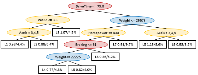
Figure 4: ReReM model tree restricted to variable types C and A for splits and A and D for regressors (Exp. R2).

cision tree part of the model tree.

• Driver related variables should only be used in the

regression expressions of the model tree.

Hence, ReReM is restricted to use conﬁguration and

assignment related variables in the decision tree and

assignment and driver related variables in the regres-

sions.

A sample tree, created using ReReM with these

settings, is presented in Figure 4. As can be seen only

variables related to conﬁguration and usage are used

in the splits. The ﬁrst split separates trucks with only

two wheel axles from the rest, which makes perfect

sense, since two axles are used on smaller trucks with

lighter assignments. Splits based on speed next sep-

arates vehicles with lower averages speed and high

fuel consumption. The fact that lower speeds indi-

cate higher fuel consumption may seem counter intu-

itive but it most likely refers to transport assignment

with very heavy loads. The remaining splits are done

based on the weight and the number of horsepower

with higher weights and more horsepower leading to

higher consumption. Finally, the regression only con-

sisted of assignment and driver related variables due

to the applied restrictions. Again, the regression ex-

pressions are not disclosed due to company policy.

The model trees created with ReReM in this exper-

iment were deemed interesting since they fulﬁlled all

requirements set by the engineers.

Table 3, shows that this setup of ReReM, i.e.,

experiment R2 drastically improves the performance

compared to the subset modeling approaches of ex-

periment S2 and R1. More speciﬁcally ReReM here

achieved substantially higher r

AND clearly lower

RMAE, compared to the manual subset modeling in

experiment S2. This increase in accuracy is much

larger than between experiment S2 and S3 and hence

the main strength of the suggest approach lies in that

much more variables can be considered while still en-

forcing relevant restrictions rather than optimizing the

subset partitioning.

Considering the complexity of the models in ex-

periment R2 and S2 both approaches were rather sim-

ilar with regard to the number of variables in the re-

gressions (19.7 vs 19.9), but ReReM consisted of 32.5

different regressions (23.5 more than in S2) thus mak-

ing the model as a whole, more complex. However,

since the subsets are created using a binary trees the

difference does not need to be so big in practice. A

balanced binary decision tree would require slightly

more than three tests on average to create the nine

subsets in experiment 1, while ﬁve would be sufﬁcient

to create the subset for the ReReM model. Hence, for

a single vehicle, the added complexity is more or less

negligible.

Another important result is how ReReM in exper-

iment R2 compares to the purely data driven approach

in D1. Interestingly enough, ReReM actually pro-

duced more accurate model trees than the purely data

driven version. In fact ReReM had a slightly higher

and a little bit lower RMAE. Obviously, the restric-

tions, had a positive effect on the predictive perfor-

mance. Since, both techniques used the same vari-

ables the difference must come from the experts rea-

soning behind the given restriction. Instead of losing

accuracy to gain the ability to act on the models, with

ReReM, interesting, i.e., actionable, models, was pro-

duced without sacriﬁcing accuracy.

6 CONCLUSION

Based on the results presented in sections 5.1 and 5.2,

it is clear that the suggested approach ReReM can cre-

ate more interesting regression and model trees by en-

forcing variable constraints.

In the ﬁrst case study concerning modeling of golf

player skill, the regression trees created using ReReM

were deemed, by a teaching professional, to be much

more interesting than a purely data driven regression

tree. The reason for the increased interestingness was

that the ReReM could be restricted to only use swing

related variables in the ﬁrst levels of the trees. With

Interesting Regression- and Model Trees Through Variable Restrictions

291

this description, it would be fairly easy for a teaching

professional to spot the deﬁciencies of the swing and

suggest drills to improves these areas. The purely data

driven model had a superior predictive performance,

compared to ReReM, but was mainly based on vari-

ables related to the ball ﬂight. Consequently, further

analysis would be required to suggest exercises and

hence the model was deemed to be less interesting.

The purpose of the second case study was to cre-

ate a better decision support for coaching of truck

drivers. Here, ReReM was compared to a manual sub-

set modelling approach often used in practice. More

speciﬁcally nine subsets were created manually us-

ing domain knowledge and statistics, based on the

average speed and total weight of the trucks. When

restricted to the same constraints as the manual ap-

proach, ReReM could increase the predictive perfor-

mance slightly by creating more subsets. An impor-

tant point is that while the manual approach is very

time consuming for human experts - at least one man-

day was needed - the corresponding task could be per-

formed within a few minutes using ReReM.

The main advantage of ReReM was, however,

demonstrated when restrictions set by engineers was

enforced. Here, the same constraints as for the man-

ual approach applied, except that more variables were

considered. In this experiment ReReM, created mod-

els with signiﬁcantly lower RMAE than the manual

approach, while still producing interesting models. In

addition, when compared to the purely data driven ap-

proach ReReM, actually had a slightly higher predic-

tive performance, while obtaining, in contrast to the

data driven approach, interesting models.

Finally, the complexity of the ReReM models was

slightly higher, i.e., the paths in the tree typically in-

cluded one or possibly two more conditions, but in

practice this would most likely be a small price to pay

for a more interesting model with high predictive per-

formance.

ACKNOWLEDGEMENTS

This work was supported by the Knowledge Founda-

tion through the project Big Data Analytics by Online

Ensemble Learning (20120192) and by Region V

astra

(VGR) under grant RUN 612-0198-13, University of

Bor

as and University of Sk

ovde.

REFERENCES

Betzler, N. F., Monk, S. a., Wallace, E. S., and Otto, S. R.

(2012). Variability in clubhead presentation charac-

teristics and ball impact location for golfers’ drives.

Journal of Sports Sciences, 30(5):439–448.

Blake, C. L. and Merz, C. J. (1998). UCI Repository of

machine learning databases.

Broadie, M. (2008). Assessing Golfer Performance Using

Golfmetrics. Science and Golf V: Proceedings of the

2008 World Scientiﬁc Congress of Golf, (1968):253–

262.

Dietterich, T. (1996). Editorial. Machine Learning,

2(24):1–3.

Fradkin, A., Sherman, C., and Finch, C. (2004). How well

does club head speed correlate with golf handicaps?

Journal of Science and Medicine in Sport, 7(4):465–

472.

Freitas, A. (2002). A survey of evolutionary algorithms for

data mining and knowledge discovery. Advances in

Evolutionary Computation, pages 819–845.

Garofalakis, M., Hyun, D., Rastogi, R., and Shim, K.

(2003). Building decision trees with constraints. Data

Mining and Knowledge Discovery, 7(2):187–214.

Grbczewski, K. and Duch, W. (2002). Heterogeneous

Forests of Decision Trees. Artiﬁcial Neural Networks

(ICANN).

Iqbal, M. R. A., Rahman, S., Nabil, S. I., and Chowdhury,

I. U. A. (2012). Knowledge based decision tree con-

struction with feature importance domain knowledge.

2012 7th International Conference on Electrical and

Computer Engineering, pages 659–662.

Iqbal, R. A. (2011). Empirical Learning Aided by Weak

Domain Knowledge in the Form of Feature Impor-

tance. 2011 International Conference on Multimedia

and Signal Processing, pages 126–130.

Lomax, S. and Vadera, S. (2013). A survey of cost-sensitive

decision tree induction algorithms. ACM Computing

Surveys, 16(2).

Nijssen, S. and Fromont, E. (2010). Optimal constraint-

based decision tree induction from itemset lattices.

Data Mining and Knowledge Discovery, 21(1):9–51.

nez, M. (1991). The use of background knowledge in

decision tree induction. Machine learning, 250:231–

250.

Quinlan, J. R. (1992). Learning with continuous classes.

In 5th Australian joint conference on artiﬁcial intelli-

gence, volume 92, pages 343–348.

Struyf, J. and Dzeroski, S. (2006). Constraint Based Induc-

tion of Multi-objective Regression Trees. 3933:222–

233.

Sweeney, M., Mills, P. M., Alderson, J., and Elliott, B. C.

(2013). The inﬂuence of club-head kinematics on

early ball ﬂight characteristics in the golf drive. Sports

Biomechanics, 12(3):247–258.

Trackman (2015). TrackMan A/S.

KDIR 2015 - 7th International Conference on Knowledge Discovery and Information Retrieval

292