Dictionary Learning: From Data to Sparsity Via Clustering

Rajesh Bhatt and Venkatesh K. Subramanian

Department of Electrical Engineering, Indian Institute of Technology Kanpur, 208016 Kanpur, India

Keywords:

Sparse Representation, Clustering, PCA, De-noising, Signal Reconstruction.

Abstract:

Sparse representation based image and video processing have recently drawn much attention. Dictionary

learning is an essential task in this framework. Our novel proposition involves direct computation of the

dictionary by analyzing the distribution of training data in the metric space. The resulting representation is

applied in the domain of grey scale image denoising. Denoising is one of the fundamental problems in image

processing. Sparse representation deals efﬁciently with this problem. In this regard, dictionary learning from

noisy images, improves denoising performance. Experimental results indicate that our proposed approach

outperforms the ones using K-SVD for additive high-level Gaussian noise while for the medium range of

noise level, our results are comparable.

1 INTRODUCTION

This paper addresses gray scale image denoising

problem in image science. Several years, re-

searchers have focused attention on this problem and

achieved continuous improvement both in terms of

performance and efﬁciency (Chatterjee and Milanfar,

2010). Surprisingly better results emerge with patch

based denoising algorithms (Elad and Aharon, 2006)

(Dabov et al., 2007). Patch based denoising algo-

rithms extract overlapping patches from a given noisy

image. Individual extracted patch were arranged in

column-wise one above other as a column vector. We

then either jointly or individually clean those patch

vectors and replace them appropriately in their cor-

responding locations in the image (Donoho et al.,

2006a).

Suppose the measured patch vector (y ∈R

) cor-

responding to the patch y ∈ R

√

n×

√

from a given

noisy image Y ∈R

N×N

,N >> n follows a y = x+ w

linear model, which estimates the original patch vec-

tor (x ∈ R

) in presence of zero mean Gaussian

noise (w ∈ R

;w ∼ N (0, σ

)) by choosing an ap-

propriate score function. For the assumed model

the maximum likelihood estimate (MLE) leads to the

mean squared error (MSE) as the optimal score func-

tion. The performance improves dramatically with

the prior knowledge of the signal. Over time, re-

searchers applied several guesses about the prior for

the images and achieved improved results. In the

Bayesian context, such priors in most cases eventually

add a regularization term in the maximum a posteri-

ori(MAP) estimate formulation. Recently, sparse rep-

resentation has emerged as a powerful prior and has

been applied to many problems including image de-

noising (Elad and Aharon, 2006), restoration (Mairal

et al., 2009), super-resolution (Yang et al., 2008),

facial image compression (Zepeda et al., 2011) and

more. In a seminal article(Elad and Aharon, 2006)

Elad et.al. proposed a new model based on sparsity

prior and it was named as Sparseland model. This

Sparseland model assumes that for an appropriate

overcomplete dictionary (D ∈ R

n×M

;n << M), tol-

erance (ε) and maximum sparsity depth L, the origi-

nal patch vector (x) can be approximately represented

as Dz. The following equations estimate the original

vector

z =argmin

kzk

Sub.to.ky−Dzk

≤ ε (1a)

x =D

z (1b)

Where, k.k

represents the L

-norm and kzk

≤L.

In (1a) ε is replaced by nCσ

, where, n is dimension

of patch vector and C represents noise gain and em-

pirically set to 1.2. Pursuit algorithms are used to

solve the non-convex optimization problem in equa-

tion (1a). Among them, orthogonal matching pur-

suit (OMP)(Tropp and Gilbert, 2007) and its vari-

ants(Donoho et al., 2006b) (Needell and Tropp, 2009)

(Needell and Vershynin, 2009) (Chatterjee et al.,

2011) achieve suboptimal solutions with excellent

trade-off between efﬁciency and computation. It has

635

Bhatt R. and K. Subramanian V..

Dictionary Learning: From Data to Sparsity Via Clustering.

DOI: 10.5220/0005573706350640

In Proceedings of the 12th International Conference on Informatics in Control, Automation and Robotics (ICINCO-2015), pages 635-640

ISBN: 978-989-758-122-9

 2015 SCITEPRESS (Science and Technology Publications, Lda.)

been shown that performance is improved by adapting

dictionary D for noisy patches, (for details see (Elad

and Aharon, 2006)). In (Aharon et al., 2006) the same

authors had proposed an elegant dictionary adapta-

tion algorithm called K-SVD and compared it with

its closest companion methods of optimal direction

(MOD) (Engan et al., 1999). Both techniques require

a set of training examples ({y

}

i=1

∈ R

) selected

from either the given noisy image or a global set of

example images and arranged in column vectors of a

matrix Y = [y

...y

]. Suppose, for the given ex-

amples, we have arranged the set of sparse represen-

tations appropriately in a matrix Z = [z

...z

For the given training matrix (Y), K-SVD dictionary

learning algorithm tries to minimize the score func-

tion (kY−DZk

), where k.k

represents Frobenius

norm. Furthermore preserves non-zero valued loca-

tion or support of each training vector’s sparse rep-

resentation corresponding to the dictionary. In each

iteration of the K-SVD algorithm, one dictionary col-

umn and the corresponding non-zero representation

coefﬁcient of all training vectors are being updated

simultaneously by doing rank-1 approximation using

singular value decomposition (SVD). The rank-1 ap-

proximation is done column-by-column using SVD,

which explains its name (for details see (Aharon

et al., 2006)). MOD (Engan et al., 1999) solves a

quadratic problem, whose analytic solution is given

by D = YZ

with Z

denoting the pseudo-inverse.

Notice that dictionary learning is a non-convex prob-

lem, hence any above technique (K-SVD/MOD) pro-

vides only a suboptimal dictionary which depends on

the initially chosen dictionary for algorithm.

In this article, we design and study a dictionary

learning scheme based on geometrical structure of

the training data selected from a given noisy im-

age. For an (N ×N) noisy image and patch size of

(

√

n×

√

n) the maximum possible number of training

data (N −

√

n + 1)

to construct a large data set. In

practice, such a huge data set is heterogeneoussince it

represents multiple different subpopulation or groups,

rather than one single homogeneous group. Cluster-

ing algorithms provides elegant ways to explore the

underlying structure of data. In the literature, some

algorithms like (Zhang et al., 2010) explore similar-

ities among patches within a local window. There-

fore, the similarity of a given patch is affected by

the chosen size of the window. It might be possi-

ble that similar patches exist outside of window. So,

we followed a simple global K-mean clustering tech-

nique. An algorithmic study of our proposed scheme

is done in section II. In section III, its effectiveness

is explored. Experimental results on several test im-

ages validate the efﬁciency of our proposed scheme

for low and high level additive Gaussian noise and

mostly surpasses the performance of denoising by a

K-SVD dictionary learning scheme. In the case of

additive medium level noise, the results are compara-

ble with the K-SVD learning scheme. The proposed

scheme can be easily extended to color image denois-

ing applications. Finally in section IV, the conclusion

and scope of further work is discussed.

2 ALGORITHM

Table 1 explains our proposed algorithm for dictio-

nary construction for denoising of an image. Let X is

an image vector and X

= R

X,i = 1,2,...N, denotes

the i

patch vector of size (

√

n×

√

n), where R

is a

matrix extracting patch X

from X. Better clustering

of similar patches can be found by using a ﬁrst round

of denoising on the patches (using the classical sparse

coding approach of Eq. (1a) presented in the previ-

ous section) before grouping them. In turn, as shown

by our experiments, our denoising output using sparse

coding approach greatly improves upon the use of this

initial denoising step.

Table 1: Algorithm.

Algorithm: Clustering Based Denoising

Task: Denoise the given image Y

Parameters: Patch Vector Size- n, Dictionary

size- M Noise Gain - C Lagrangian Multiplier-

λ, Number of Clusters-K and Hard Threshold

-ing Parameter T

Initialization: N-Examples patches from

Execute One time:

• Cleaning: Use pursuit algorithm (OMP)

to clean N-example vectors

• Clustering: Apply clustering algorithm (K-

means) to cluster cleaned example vectors

• Dictionary: For each cluster, all non-zero

eigen value principal components (PCs) are

cascaded in D matrix

• Averaging: Set

X using below equation as

in (Elad and Aharon, 2006). R

i, j

Y represents

patch vector corresponding to (i, j) top left

patch location in

X = (λI +

∑

i, j

)

−1

(λ

Y+

∑

i, j

)

Once cleaning of patches is done, K-means clus-

tering algorithm is applied to get similar patches in re-

spective groups. Here K-means is used due to the sim-

plicity of the algorithm. Afterwards PCA (principal

component analysis) is applied to respective cluster

ICINCO2015-12thInternationalConferenceonInformaticsinControl,AutomationandRobotics

636

Table 2: Summary of the PSNR result in decibels. In each cell, two results are reported. Left: K-SVD trained dictionary.

Right: PCA trained dictionary. All reported results are average over 20 experiments.

σ/PSNR Lena Pepper Camera Lake Bridge Ship

2/42.110 43.599 43.486 43.247 43.161 46.693 46.268 43.167 43.099 42.689 42.668 43.134 43.081

5/34.164 38.524 38.535 37.793 37.623 41.375 40.899 36.873 36.872 35.771 35.805 37.119 37.108

7/31.236 37.07 36.978 36.189 36.044 39.505 39.022 34.91 34.947 33.429 33.509 35.339 35.284

20/22.102 32.405 32.008 32.207 31.817 33.376 32.867 29.984 29.68 27.377 27.206 30.388 29.918

40/16.062 28.981 28.635 29.203 28.716 29.702 29.252 26.715 26.286 24.243 23.999 27.05 26.585

60/12.571 26.838 26.649 26.979 26.661 27.599 27.042 24.709 24.441 22.685 22.525 25.086 24.783

100/8.117 24.498 24.467 24.233 24.174 24.151 23.921 22.349 22.299 21.19 21.162 22.753 22.678

140/5.227 22.972 23.013 22.687 22.704 22.242 22.254 21.057 21.067 20.276 20.282 21.558 21.583

160/4.056 22.313 22.369 21.963 22.021 21.685 21.7 20.605 20.626 19.971 19.993 21.086 21.12

180/3.026 21.719 21.783 21.336 21.39 21.056 21.105 20.208 20.251 19.585 19.611 20.75 20.801

200/2.117 21.161 21.254 20.903 20.990 20.535 20.593 19.714 19.778 19.221 19.276 20.188 20.258

patch vectors. All the eigenvectors from the clusters

are cascaded to form dictionary. Finally every patch

vector from the original noisy image is transformed

to sparse domain using the dictionary. Sparse code

is found using OMP until the reconstruction error is

above the threshold. Using the sparse code, the corre-

sponding patch vector is reconstructed and averaging

as shown in equation is applied. We have used over-

lapping patch vector from the noisy image to avoid

blocking artifacts.

3 RESULTS

In present section, we show the results achieved by

applying mentioned methods on several standard test

images with two dictionary learning techniques. In

order to enable a fair comparison, test images as well

as noise levels are same as used in denoising exper-

iments reported in (Elad and Aharon, 2006). Exper-

imental evidences suggested that except very fewer

cases overcomplete/redundant DCT (ODCT) dictio-

nary has inferior performance among three methods.

One such case is shown in ﬁgure ??. However, other

methods eventually perform better as dictionary col-

umn size increases. Further, detailed discussion on

effect of dictionary size is done at end of present sec-

tion. Table 2 summarizes denoising results of pro-

posed and K-SVD based dictionary learning from cor-

rupted images. Furthermore, experiments are con-

ducted for various test images and for set of noise

parameter (σ) values. Every result reported is an av-

erage over 20 experiments, having different realiza-

tions of noise with ﬁxed parameter value σ in each

trial. The redundant DCT dictionary is obtained by

applying Kronecker product on square DCT matrix.

Furthermore, this redundant dictionary was also used

as initialization for learning K-SVD based dictionary.

The output of K-SVD trained dictionary is shown

on the bottom-left of Fig 2. Notice that all training

patches vectors were generated from uniform sam-

pling of given noisy image in overlapped manner.

In all experiments, the denoising process included a

sparse-coding of each patch of size 8 by 8 pixels from

the noisy image. Using the OMP, atoms were accu-

mulated till the average error passed the threshold,

chosen to be 1.20σ as suggested in (Elad and Aharon,

2006). The denoised patches were averaged, as de-

scribed in (Elad and Aharon, 2006).

A simulation is done for the proposed algorithm

for different numbers of clusters (1,4,9 and 16) result-

ing in corresponding dictionary sizes of 64, 256, 574

and 1024 respectively. Experimentally we have found

that performance almost saturates after dictionary size

greater than 256, therefore all result in table 2 and ﬁg-

ure 1 shown for dictionary size 256.

It is clear from Table 2, performance of different

algorithmsare closed. Average PSNR of denoised im-

age using proposed algorithm for noise level less than

σ = 7 performs better than both ODCT and K-SVD

based dictionary learning approach. Results corre-

sponding to proposed algorithm for noise levels 2 are

better than K-SVD. For mid level noise the proposed

approach performs slightly lower then K-SVD. For

higher noise power, experiments demonstrated better

performance of proposed method then other methods.

In order to better visualize the results and compar-

ison, Fig. 4 presents the difference of the denois-

ing results of the proposed methods and the overcom-

plete DCT. Similarly difference between K-SVD and

ODCT is plotted. Both are compared with that of a

zero straight reference line. This comparison is pre-

sented for the images Lena, Peppers, Camera, Lake,

Bridge and Ship. Notice that, for these images, the

proposed dictionary performs better than the reported

DictionaryLearning:FromDatatoSparsityViaClustering

637

0 50 100 150

−1

−0.5

0.5

Sigma

Difference in dB

Base for comparison

PCA

KSVD

(a)

0 50 100 150

−1

−0.5

0.5

Sigma

Difference in dB

Base for comparison

PCA

KSVD

(b)

0 50 100 150

−1

−0.5

0.5

Sigma

Difference in dB

Base for comparison

PCA

KSVD

(c)

0 50 100 150

−1

−0.5

0.5

Sigma

Difference in dB

Base for comparison

PCA

KSVD

(d)

Figure 1: Comparison between the two methods: K-SVD based dictionary trained on patches from the noisy image and our

proposed approach results shown for four test images.

(a) (b)

Figure 2: Denoising results for the image Lena corrupted with additive Gaussain noise, σ = 20. (a). The original Lena image.

(b). The noisy image. (c). Denoised image using K-SVD. (d). Denoised image using our proposed approach.

ICINCO2015-12thInternationalConferenceonInformaticsinControl,AutomationandRobotics

638

(a) (b)

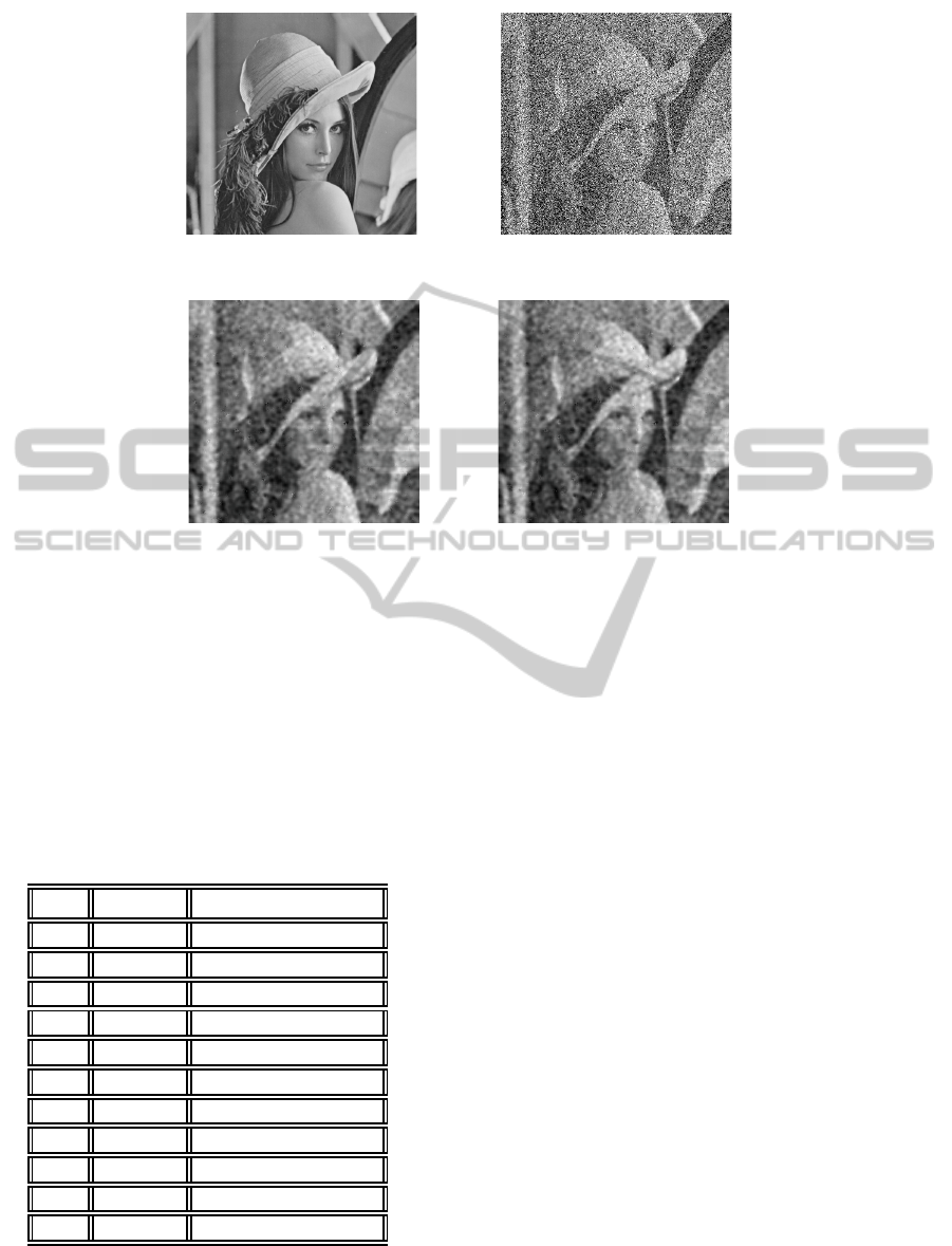
Figure 3: Denoising results for the image Lena corrupted with additive Gaussain noise, σ = 180. (a). The original Lena image.

(b). The noisy image. (c). Denoised image using K-SVD. (d). Denoised image using our proposed approach.

results of K-SVD for noise levels greater than 100,

while the ODCT dictionary often achieves very close

results. In the image Barbara, however, which con-

tains high-frequency texture areas, the adaptive dic-

tionary that learns the speciﬁc characteristics has a

clear advantage over the proposed dictionary.

Table 3: Time taken in denoising by K-SVD algorithm and

proposed approach at various σ values.

σ K-SVD Proposed Approach

2 149.296 69.939

5 57.083 54.823

7 39.033 53.230

20 14.389 54.414

40 9.414 60.875

60 8.280 64.123

100 7.498 49.755

140 7.367 49.152

160 7.267 49.646

180 7.302 49.206

200 7.344 49.677

The system used for simulation is Intel(R)

Core(TM) i7-2600 CPU @ 3.40GHz, 4GB RAM,

running on Windows 7. Programming language used

is MATLAB. Time taken by K-SVD and our pro-

posed approach for denoising is calculated for differ-

ent sigma values of noise. As can been seen clearly

from Table 3 for smaller values of σ our proposed ap-

proach takes very less time as compared to K-SVD

based denoising method. As the σ value increases

time taken by both our proposed approach and K-

SVD decreases. This decrease in time is expected

as the threshold while calculating sparse code using

OMP increases (threshold is directly proportional to

σ.). As σ increases time taken by K-SVD decreases at

sharper rate than our proposed approach. This behav-

ior is also expected as OMP is used in K-SVD during

dictionary learning and not in our proposed approach.

To conclude this experimental section, we refer to

our arbitrary choice of dictionary atoms (this choice

had an effect over all three experimented methods).

We conducted another experiment, which compares

between several values of the number of clusters k.

In this experiment, we tested the denoising results of

the three proposed methods on the image House for

an initial noise level of sigma value 15. The tested

dictionary size were 64, 128, 256, and 512. As can

be seen, the increase of the number of dictionary el-

ements generally improves the results, although this

improvement is small.

DictionaryLearning:FromDatatoSparsityViaClustering

639

200 400 600 800 1000

29.9

30.1

30.2

30.3

30.4

# Dictionary Elements (K)

Average PSNR (in dB)

Proposed

ODCT

KSVD

Figure 4: Effect of changing the number of dictionary ele-

ments (k) on the ﬁnal denoising results for the image House

and for sigma = 15.

4 CONCLUSION

In this paper, a novel, intuitively appealing dictionary

construction algorithm has been developed which

achieves performance comparable to the K-SVD ap-

proach at medium noise levels, and visibly better

PSNR for high levels of noise in the denoised im-

age. The algorithm developed is intuitive and efﬁ-

cient. The work presented here has been compared to

the state of the art technique of image denoising.

REFERENCES

Aharon, M., Elad, M., and Bruckstein, A. (2006). K-svd:

An algorithm for designing overcomplete dictionaries

for sparse representation. IEEE Transaction on Signal

Processing, 54(11):4311–4322.

Chatterjee, P. and Milanfar, P. (2010). Is denoising dead?

IEEE Transactions on Image Processing, 19(4):895 –

911.

Chatterjee, S., Sundman, D., and Skoglund, M. (2011).

Look ahead orthogonal matching pursuit. In IEEE

Int. Conf. Acoustics Speech and Signal Processing

(ICASSP).

Dabov, K., Foi, A., Katkovnik, V., and Egiazarian, K.

(2007). Image denoising by sparse 3-d transform-

domain collaborative ﬁltering. IEEE Transactions on

Image Processing, 16(8):2080 –2095.

Donoho, D., Elad, M., and Temlyakov, V. (2006a). Stable

recovery of sparse overcomplete representations in the

presence of noise. IEEE Transactions on Information

Theory, 52(1):6 – 18.

Donoho, D., Tsaig, Y., Drori, I., and Starck, J. (2006b).

Sparse solution of underdetermined linear equations

by stagewise orthogonal matching pursuit. Technical

report.

Elad, M. and Aharon, M. (2006). Image denoising via

sparse and redundant representations over learned dic-

tionaries. IEEE Transactions on Image Processing,

15(12):3736 –3745.

Engan, K., Aase, S. O., and Hakon Husoy, J. (1999).

Method of optimal directions for frame design. In

Proceedings ICASSP’99 - IEEE International Con-

ference on Acoustics, Speech, and Signal Processing,

volume 5, pages 2443–2446.

Mairal, J., Bach, F., Ponce, J., Sapiro, G., and Zisserman,

A. (2009). Non-local sparse models for image restora-

tion. In IEEE 12th International Conference on Com-

puter Vision, pages 2272 –2279.

Needell, D. and Tropp, J. (2009). Cosamp: Iterative sig-

nal recovery from incomplete and inaccurate samples.

Appl. Comput. Harmon. Anal., 26(3):301–321.

Needell, D. and Vershynin, R. (2009). Uniform uncertainty

principle and signal recovery via regularized orthogo-

nal matching pursuit. Found. Computational Mathe-

matics, 9:317–334.

Tropp, J. and Gilbert, A. (2007). Signal recovery from

random measurements via orthogonal matching pur-

suit. IEEE Transactions on Information Theory,

53(12):4655–4666.

Yang, J., Wright, J., Huang, T., and Ma, Y. (2008). Image

super-resolution as sparse representation of raw image

patches. In IEEE Conference on Computer Vision and

Pattern Recognition(CVPR), 2008, pages 1 –8.

Zepeda, J., Guillemot, C., and Kijak, E. (2011). Im-

age compression using sparse representations and the

iteration-tuned and aligned dictionary. IEEE Journal

of Selected Topics in Signal Processing,, 5(5):1061 –

1073.

Zhang, L., Dong, W., Zhang, D., and Shi, G. (2010). Two-

stage image denoising by principal component anal-

ysis with local pixel grouping. Pattern Recognition,

43(4):1531 – 1549.

ICINCO2015-12thInternationalConferenceonInformaticsinControl,AutomationandRobotics

640