
Comparison of Controllable Transmission Ratio Type Variable
Stiffness Actuator with Antagonistic and Pre-tension Type Actuators
for the Joints Exoskeleton Robots
Hasbi Kizilhan, Ozgur Baser, Ergin Kilic and Necati Ulusoy
Süleyman Demirel University, Mechanical Engineering Departmant, Isparta, Turkey
Keywords: Exoskeleton Robots, Variable Stiffness Actuators, Controllable Transmission Ratio Type Actuators,
Antagonistic Type Actuators, Pre-tension Type Actuators.
Abstract: Exoskeleton robots are used as assistive limbs for elderly persons, rehabilitation for paralyzed persons or
power augmentation purposes for healthy persons. The similarity of the exoskeleton robots and human body
neuro-muscular system maximizes the device performance. Human body neuro-muscular system provides a
flexible and safe movement capability with minimum energy consumption by varying the stiffness of the
human joints regularly. Similar to human body, variable stiffness actuators should be used to provide a
flexible and safe movement capability in exoskeletons. In the present day, different types of variable
stiffness actuator designs are used, and the studies on these actuators are still continuing rapidly. As
exoskeleton robots are mobile devices working with the equipment such as batteries, the motors used in the
design are expected to have minimal power requirements. In this study, antagonistic, pre-tension and
controllable transmission ratio type variable stiffness actuators are compared in terms of energy efficiency
and power requirement at an optimal (medium) walking speed for ankle joint. In the case of variable
stiffness, the results show that the controllable transmission ratio type actuator compared with the
antagonistic design is more efficient in terms of energy consumption and power requirement.
1 INTRODUCTION
Human neuro-musculo-skeletal system achieves a
flexible and stable walking with minimum energy
consumption by changing the stiffness and damping
in lower limb joints. The design of exoskeleton
robots employing variable stiffness actuators (VSA)
has been introduced to the literature in recent time.
As exoskeleton robots are mobile robots and
interacting with human limbs, variable stiffness
actuators used in their designs need to be energy
efficient and safe. Utilizing stiff actuators (electricity
motor and hydraulic actuators etc.) on these robots is
not appropriate to increase safety and provide
biomimetic motion. Instead, novel promising
designs of variable stiffness actuators are needed to
achieve the desired criteria. Due to the significant
properties of the variable stiffness actuators like
minimizing large shock forces, safely interacting
with the user and storing/releasing energy in their
passive elastic elements, the use of them on the
exoskeleton robots is increasing more and more.
Therefore, the studies on novel actuator designs are
still continuing rapidly. There are some important
design criteria for VSAs. They can be summarized
as follows: (1) variable stiffness actuators should be
compact and light, (2) stiffness range of the
actuators should be wide as possible in order to
employ them in many applications, (3) stiffness of
the actuators should be changed rapidly, (4) they
should have a minimum level of power requirement,
(5) both equilibrium position and stiffness of the
actuators should be adjusted independently.
Variable stiffness actuator designs (compliant
actuators) have considerable advantages such as
storing/releasing energy by means of the passive
elastic elements used in their structure, safely
interacting with the users and minimizing the large
shock forces (Alexander, 2010). Therefore, they are
started to use in the robots interact with human and
humanoid robots. Nowadays, the studies for more
efficient, more compact and lighter new actuator
designs are still carrying on. These actuators are
classified under five different categories. These are
equilibrium-controlled, antagonistic-controlled,
structure-controlled, mechanically controlled and
188
Kizilhan H., Baser O., Kilic E. and Ulusoy N..
Comparison of Controllable Transmission Ratio Type Variable Stiffness Actuator with Antagonistic and Pre-tension Type Actuators for the Joints
Exoskeleton Robots.
DOI: 10.5220/0005507801880195
In Proceedings of the 12th International Conference on Informatics in Control, Automation and Robotics (ICINCO-2015), pages 188-195
ISBN: 978-989-758-123-6
Copyright
c
2015 SCITEPRESS (Science and Technology Publications, Lda.)
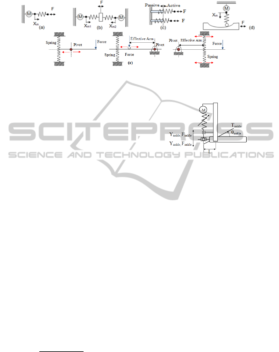
Figure 1: Variable stiffness actuator types: (a) equilibrium-controlled, (b) antagonistic-controlled, (c) structure-controlled,
(d) mechanically-Controlled and (e) controllable transmission ratio type actuators.
controllable transmission ratio type actuators (Van
Ham, 2007; Vanderborght, 2012). Figure 1 shows
their schematic views. Some implementations of
these actuators are presented in the references (Pratt,
1995; Migliore, 2005; Hollander, 2006; Jafari, 2010;
Jafari, 2011).
2 CONTROLLABLE
TRANSMISSION RATIO TYPE,
ANTAGONISTIC AND
PRE-TENSION ACTUATOR
DESIGNS
In this section, all equations are derived to compare
antagonistic, pre-tension and controllable
transmission ratio type actuators in a simulation
study. Firstly, it is assumed that the actuators are
designed linearly, and thus the linear motion of the
actuators need to be transformed into the rotary
motion for lower limb joints. Besides,
biomechanical moment and angle data cannot be
used directly for linear actuator designs. They
should be converted for linear actuator designs
according to the mechanism used in the design. A
slider-moment arm mechanism can be used for that
purpose. Figure 2 shows a schematic drawing of that
mechanism applied on the ankle joint so that the
rotary motion of the ankle joint can be transformed
to a linear motion. The transformation equation of
that mechanism can be derived as Eq.(1) by using
the trigonometric relation between the ankle joint
axis and force application point of the linear
actuator.
=
(1)
,
,
,
in the equations represent
ankle joint angle, ankle joint moment, vertical
deflection of the linear actuator and output force of
the linear actuator, respectively.
Figure 2: Slider-moment arm mechanism of a linear
variable stiffness actuator used in an ankle joint.
2.1 Controllable Transmission Ratio
Type Actuator
The stiffness of this type of actuator design is
adjusted by changing the transmission ratio between
the spring and output link. One motor (M2) performs
this stiffness adjustment and another motor (M1)
only controls the equilibrium position of the whole
mechanism. In this arrangement, as the spring is not
forced, no energy is required to change the stiffness
of the design. In the design of controllable
transmission ratio type actuators presented in this
paper, the pivot point and spring position are
stationary and the position of the force output link is
controlled, and thus the stiffness of the actuator can
be tuned to a desired value. Figure 3 shows the
schematic view of the presented design. The
equivalent output stiffness characteristics of the
variable stiffness actuators is desired to be almost
linear, so that the elastic elements used in this design
need to be linear spring.
As the spring elements used in the design are
linear springs, the force output of the actuator can be
formulated as Eqs. (2) and (3). The positon of the
force output link on the lever arm is changed to
adjust the transmission ratio in the controllable
transmission ratio type actuator. Figure 4 shows the
free body diagram of the lever arm used in the
design.
ComparisonofControllableTransmissionRatioTypeVariableStiffnessActuatorwithAntagonisticandPre-tensionType
ActuatorsfortheJointsExoskeletonRobots
189
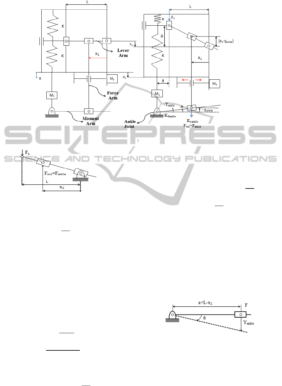
Figure 3: Schematic view of a controllable transmission ratio type actuator.
Figure 4: Free body diagram of the lever arm.
=
=
(2)
=
(3)
,
, L and
in this equation represent the
output force of variable transmission mechanism,
spring force, horizontal length of the lever arm and
the distance between the pivot point and output force
link, respectively. Eq.(4) represents the spring force;
=2
(4)
K and Δ in this equation represent the linear spring
constant and deflection of springs. Substituting Eq.
(4) into the Eq. (3), the output force of the actuator
and deflection of the spring can be formulated as
Eqs. (5) and (6), respectively.
=
2
(5)
=
(6)
Substituting Eq. (5) into Eq. (6), output force of the
actuator can be expressed as follow;
=2.
(7)
Output force of the actuator is also called as ankle
force in the paper. By solving Eq. (2) and (7) in
common, the stiffness on the output link (force arm)
of the linear actuator can be formulated as Eq. (9);
=2
(8)
=2
(9)
The relation between the ankle force applied by the
actuator force arm and ankle moment on the moment
arm is depicted in Figure 5. (a+L-x
2
) on the figure
represents the effective length of the moment arm,
and a and L distances are constant according to the
controllable transmission ratio type actuator design
as shown in Figure 3. x
2
represents the required
distance between the output link and pivot point to
adjust the stiffness. Besides, θ and y
ank
represent the
ankle joint angle and vertical deflection of the force
arm of the actuator, respectively.
Figure 5: Moment arm mechanism of the ankle joint.
Trigonometric relation between vertical deflection of
the force arm (y
ank
) and ankle joint angle (y
ank
) can
be written as Eqs. (10) and (11) by considering
Figure 5.
ICINCO2015-12thInternationalConferenceonInformaticsinControl,AutomationandRobotics
190
=
(10)
=
(11)
Also, the relation between the output force of the
actuator (ankle force) and ankle moment can be
written as Eqs. (12) and (13);
=
(12)
=
(13)
Substituting the trigonometric equation, Eq. (11),
into Eq. (13), ankle moment can be rewritten as;
=
(14)
Also, substituting Eq. (9) into Eq. (14) for
, the
ankle moment can be expressed more clearly as Eq.
(15);
=2
2
(15)
Differential equation of this ankle moment
formulation in terms of θ gives the rotational
stiffness of the ankle joint;
=
=2
(16)
As given in Eq. (17),
can be derived from Eq.
(16). This equation can be used to calculate the
required position of the output link to be controlled
by the second motor (M2) for ankle joint stiffness
adjustment.
=
.
(17)
Besides, Eq. (18) can be used to calculate the
required position of the main motor (M1) for
providing ankle joint moment;
=
(18)
Substituting Eq. (9) into Eq. (18) for
, the
required equilibrium position of the controllable
transmission ratio type actuator to be controlled by
the main motor (M1) can be rewritten as Eq. (19);
=
.
(19)
Moreover, Substituting Eq. (10) into the Eq. (19) for
, the general form of the required equilibrium
position of the actuator can be derived as Eq. (20);
=
.
2
(20)
Then, substituting Eqs. (20) and (10) into Eq.(8), the
force applied by the main motor can expressed as
Eq. (21);
=2
.
(21)
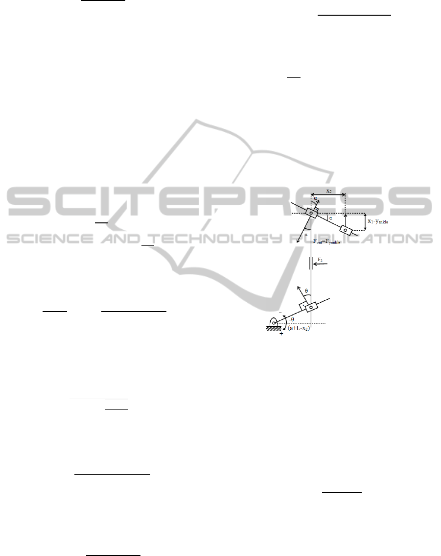
The geometric relation between the spring side and
ankle side of the force arm should be considered to
calculate the force applied by the second motor
(M2), and the free body diagram of the force arm is
shown in Figure 6. In the figure, α and θ angles
represent the angles between lever arm and force
arm on the spring side, and between moment arm
and force arm on the ankle joint side, respectively.
Figure 6: Free body diagram for the force arm of the
controllable transmission ratio type actuator.
The sum of the horizontal forces can be equalized on
the force arm (
∑
=0) to calculate the force
applied by the second motor (F
2
). Thus, it can be
formulated as Eq. (22);
=
cos.sincossin
(22)
In this equation, is equal to ankle joint angle and α
can be expressed as Eq. (23) by considering the
geometry on the free body diagram;
=tan
(23)
Finally, the total power requirement and total energy
consumption of the controllable transmission ratio
type actuator can be calculated by using Eqs. (24)
and (25). The first and second terms of these
equations represent the power requirement and
energy consumption of the first and second motor,
respectively. These equations will also be used to
calculate the power requirement and energy
ComparisonofControllableTransmissionRatioTypeVariableStiffnessActuatorwithAntagonisticandPre-tensionType
ActuatorsfortheJointsExoskeletonRobots
191
consumption of the other designs.
=
=
.
.
(24)
=
|
|
|
|
(25)
2.2 Antagonistic Type Actuator
Two different series elastic actuators are connected
with facing one another in the antagonistic design. In
this design, the stiffness and the equilibrium point of
the actuator could be adjusted by non-linear springs,
which are simultaneously controlled by two different
motors. The equivalent stiffness output
characteristics of the variable stiffness actuators are
desired to be linear. Therefore, quadratic non-linear
springs should be used in the design of antagonistic
type variable stiffness actuators for the linear
adaptable compliance.
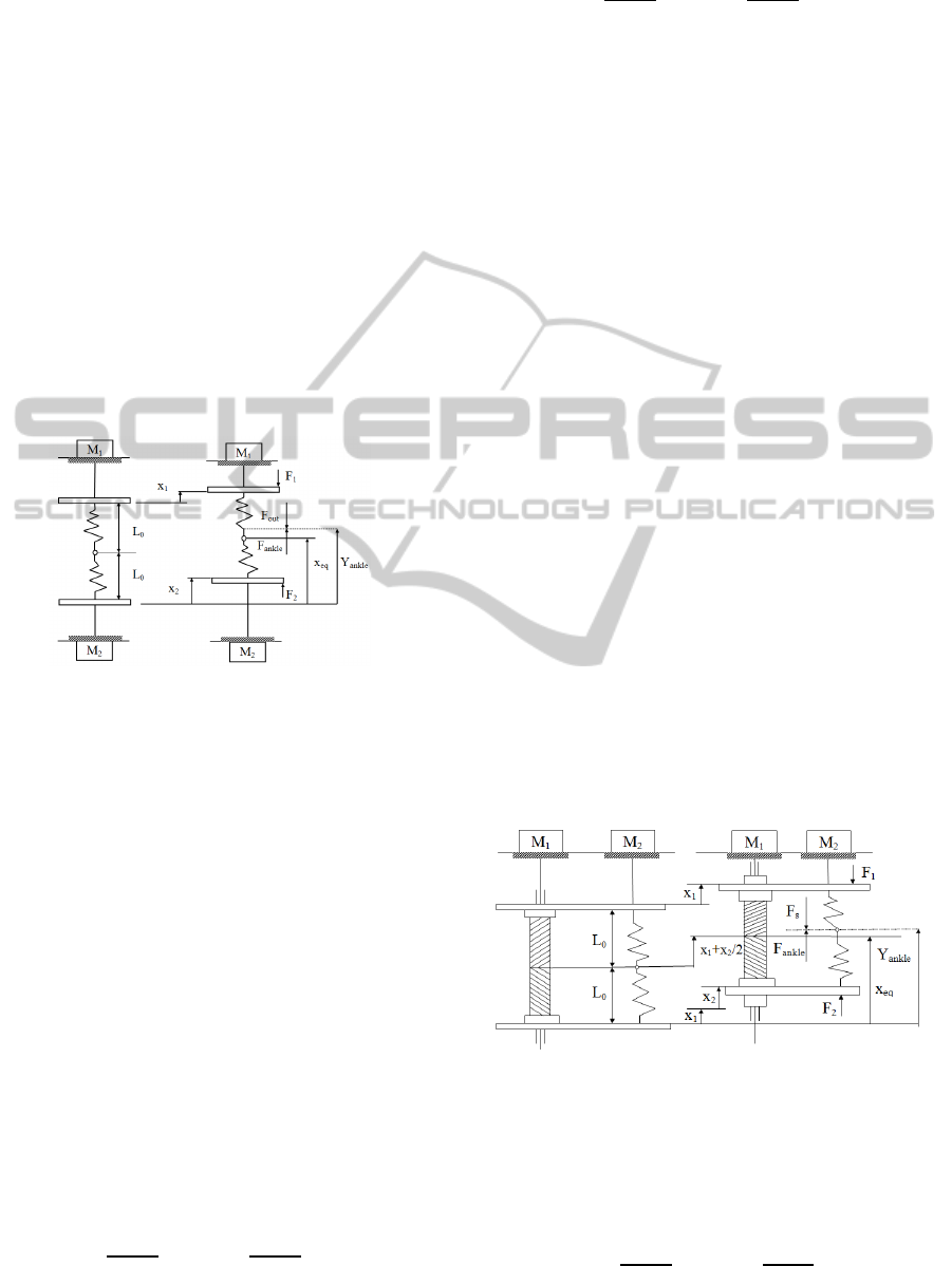
Figure 7: Schematic view of a linear antagonistic type
variable stiffness actuator.
Figure 7 depicts a schematic view of a linear
antagonistic design. Referring to Figure 7,
is the
equilibrium position of the actuator,
is the linear
displacement of ankle joint on the antagonistic type
actuator. Also,
,
,
,
, F
1
, F
2
, x
1
,
x
2
,
represents the equilibrium position of the
actuator, position of the ankle, output force of the
linear actuator, reaction force created by ankle over
the actuator, force applied by the first motor, force
applied by the second motor and free length of the
springs used in the design, respectively. Under the
assumption of that the springs are quadratic, ankle
force will be equal to the difference of the forces
created by the motors. Similar to the previous
derivations, the positions and forces of the first and
second motors are derived as Eqs. (26-29),
respectively. The symbol K shows the stiffness rate
of the quadratic spring model used in the
antagonistic design
=.
.
=
4
(26)
=
4
(27)
=
2
(28)
=
(29)
2.3 Pre-tension Type Actuator
In the design of the pre-tension actuator (another
name mechanically-controlled actuator) which is
taken as an example in this study, there are two non-
linear springs which are connected opposed to each
other and compressed by only a one motor (M1).
Therefore, the stiffness of the actuator on the
connection point of the springs could be consistently
adjusted by M1 and the second motor (M2) will be
used to control the equilibrium point of the whole
system. A schematic view is given in Figure 8 to
figure out the pre-tension design example used in
this study. In this schematic design example, M1
drives the twin ball-screw mechanism with double
nut and compresses the opposed springs at the same
amount. Therefore, the stiffness of the actuator could
be easily changed by the equal displacement of the
(quadratic) non-linear springs.
In Figure 8,
,
,
,
, F
1
, F
2
, x
1
,
x
2
,
represents the equilibrium position of the
actuator, position of the ankle, output force of the
linear actuator, reaction force created by ankle over
the actuator, force applied by the first motor, force
applied by the second motor and free length of the
springs used in the design, respectively. Note that
the springs used in the pre-tension design were also
quadratic
=.
.
Figure 8: Schematic view of a pre-tension type variable
stiffness actuator example.
With the similar derivations presented in the
previous sections, the positions and forces of the
first and second motors are derived as Eqs. (30-33),
respectively.
=
4
(30)
ICINCO2015-12thInternationalConferenceonInformaticsinControl,AutomationandRobotics
192
=
2
(31)
=
(32)
=
4
(33)
3 SIMULATION AND
DISCUSSION
In this section, simulation results are presented in the
case of in using ankle joint of antagonistic, pre-
tension, controllable transmission type actuator
designs and the results with these simulations are
given. Before starting the simulation studies,
biomechanics data are needed for the ankle with
which the designs will be tested.
There are many biomechanic studies concerning
human beings’ lower body joints in the literature. In
these studies, the walking patterns in different
individuals’ walking speed levels are observed by
using markers positioned in joints and cameras.
Thus, lower body joints’ angles, speed and
acceleration levels are obtained by processing these
patterns. Furthermore, the mass and inertia of lower
body joints for people with specific height and
weight are also presented in the books related with
biomechanics. Moment and power graphics for
lower body joints during walking can be calculated
by using angles, speed and acceleration levels
obtained from the walking experiments in reverse
dynamic equations.
Firstly, biomechanics data are needed for the
angle and moment values of the ankle in simulation
studies. The data provided by Bovi et al. study on
bio-mechanics have been used in this study (Bovi,
2010). According to these data, ankle position angle
and moment values of an optimum walking speed
(0.8 ≤ walking speed/height ≤ 1) of an average adult,
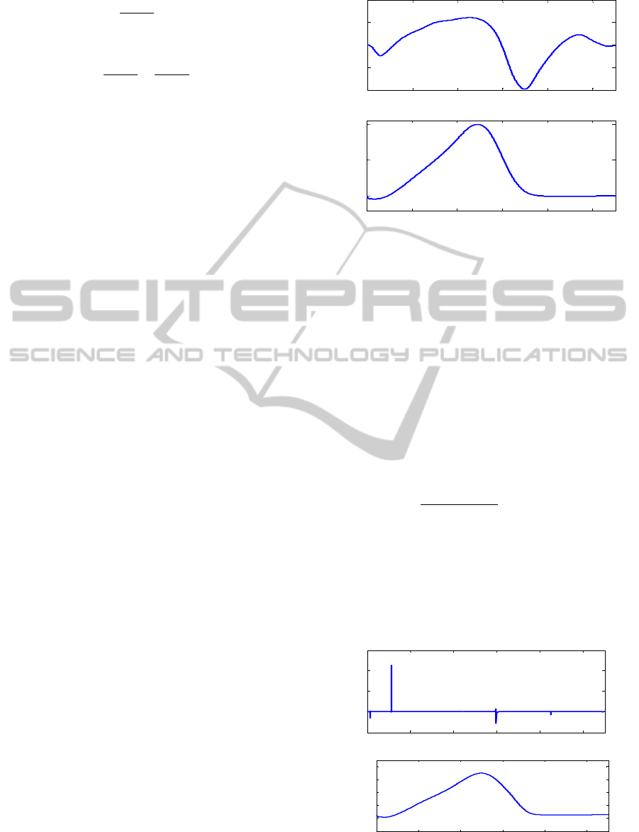
with 80 kg weight, are shown in Figure 9.
When the moment values given in Figure 9 are
divided to the ankle angle values, in order to
calculate the stiffness values of the ankle during
walking, shown in Figure 10 have provided a
stiffness value, which is really hard to happen. If
these values are wanted to be obtained by any
actuator whose stiffness can be changed, actuators,
which can reach high stiffness values in a very short
time, are required. This is really hard to apply, since
it requires high levels of power. Therefore, Holgate
et al. proposed to modify this stiffness graphic
(Holgate, 2008).
Figure 9: (a) Ankle angle and (b) ankle moment during
one walking cycle.
This study aims to have reachable stiffness values by
offsetting the ankle angle according to the
recommended method. Stiffness value is near zero
while the ankle is in swing phase in this method
recommended by Holgate et al. It is inevitable to
have unwanted oscillations when the stiffness value
is zero in the swing phase of the ankle. Therefore, it
is possible to prevent these unwanted oscillations by
adding a second offset to the stiffness value
obtained. Thus, the data in Figure 9 and the modified
stiffness values obtained by using Eq.34 are
obtained as given in Figure 10 (b).
=
(34)
In Eq.34,
shows the stiffness value of the
ankle to be used in the simulations,
,
,
,
and A represent the moment of the
ankle, the angle of the ankle, the offsetting in the
angle of the ankle, the modified stiffness value of
the ankle and tuning multiplier, respectively.
Figure 10: (a) Calculated stiffness values, (b) Modified
stiffnesss values.
0 0.2 0.4 0.6 0.8 1 1.1
-0.4
-0.2
0
0.2
0.4
Ankl e Posi t i on (rad. )
Time (s )
(a)
0 0,2 0,4 0,6 0,8 1 1,1
0
50
100
Tim e (s )
Ankl e Moment (N-m)
(b)
0 0.2 0.4 0.6 0.8 1 1.1
-1
0
1
2
3
x 10
5
Tim e (s )
Ankl e St i f f ness (Nm/ r ad. )
(a)
0 0.2 0.4 0.6 0.8 1 1.1
0
200
400
600
800
1000
Time (s )
Ankl e Stiffness (Nm/rad. )
(b)
ComparisonofControllableTransmissionRatioTypeVariableStiffnessActuatorwithAntagonisticandPre-tensionType
ActuatorsfortheJointsExoskeletonRobots
193
Obtaining the equation for the design of
antagonistic, pre-tension and controllable
transmission type actuator designs has been
described in detail in Section 2.
Simulation tests for three different design have
been run by using these equations in MATLAB
Simulink
®
. In these simulation studies, the modified
stiffness value given in Figure 10 (b) and ankle
angle and torque values given in Figure 9 are taken
as reference values. In the study for antagonistic and
pre-tension actuators, quadratic spring model, and in
the study for controllable transmission type actuator
a linear spring model are used. Spring rate
coefficients for quadratic and linear springs are
taken to be K
rate
=800 kN/m
2
and 3000 kN/m
respectively. At the same time, slider-moment arm
mechanism of a linear variable stiffness actuator
used in an ankle joint was taken as (L) 10 cm.
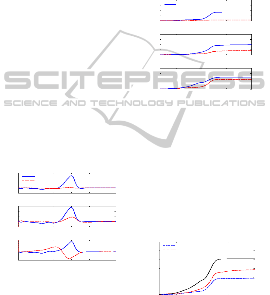
In Figures 11 and 12, power requirement of
motors used in each design and the amount of the
energy spent by motors are presented. As can be
analyzed power graph given in Figure 11, while in
these three designs the first motors need 250W
power, the second motors have quite different power
needs. According to the reference simulation
scenario, while in the antagonistic and pre-tension
designs, second motor needs 100W power
requirement, in the controllable transmission type
actuator design needs 10W power requirement.
Therefore, it is possible to work with smaller motors
in the controllable transmission type actuator design.
Figure 11: Power requirement; (a) controllable
transmission type (b) antagonistic and (c) pre-tension type
actuator designs.
In Figure 12, the energy levels consumed by motors
similar to the graphics of power requirement are
presented. As in power requirement graphics, even
though the first motors of each three designs have
similar energy consumption, there are significant
differences in the second motors’ energy
consumption. The second motors consume 40J
energy in pre-tension design, 15J energy in
antagonistic design and about 3J energy in the
controllable transmission type actuator design.
Figure 12: Consumed energy: (a) controllable transmission
type (b) antagonistic and (c) pre-tension type actuator
designs.
Lastly, for all three designs, the total energy
consumed by motors are given in Figure 13. This
graphic shows 80J energy in pre-tension design, 55J
energy in antagonistic design and 37J energy in the
controllable transmission type actuator design have
been consumed during a walking cycle of an 80 kg
person with the optimum speed (average speed) and
the scenario of walking on a flat ground. The energy
consumption difference between controllable
transmission type actuator design and the other two
designs are quite important for mobile human-like
robots operated by batteries. Therefore, it concluded
that in terms of energy consumption, it is much
better to use controllable transmission type actuator
design in exoskeleton robots.
Figure 13: Total energy consumption.
0 0.2 0.4 0.6 0.8 1
-100
0
100
200
300
Time (s )
Power (Watt)
0 0.2 0.4 0.6 0.8 1
-100
0
100
200
300
Time (s )
Power (Watt)
0 0.2 0.4 0.6 0.8 1
-200
0
200
300
Time (s )
Power (Watt )
Moto r - 1 Po w er
Moto r - 2 Po w er
(b)
(c)
(a)
0 0.2 0.4 0.6 0.8 1
0
20
40
60
80
Time (s)
Energy (Joul e)
Motor-1 Energy
Motor-2 Energy
0 0.2 0.4 0.6 0.8 1
0
20
40
60
80
Time (s)
Energy (Joul e)
0 0.2 0.4 0.6 0.8 1
0
20
40
60
80
Time (s)
Energy (Joul e)
(a)
(b)
(c)
0 0.2 0.4 0.6 0.8 1
0
20
40
60
80
100
120
Tot al Energy Consumpti on (Joule)
Tim e (s )
Controllable Transmission
Antagonistic
Pretension
ICINCO2015-12thInternationalConferenceonInformaticsinControl,AutomationandRobotics
194

4 CONCLUSIONS
In this study, first of all, equilibrium-controlled
actuator, antagonistic-controlled actuator, structure-
controlled actuator, mechanically-controlled actuator
and controllable transmission ratio type actuator
designs are presented in detail. Then, all equations
have been derived for the design of an antagonistic,
pre-tension and controllable transmission ratio type
actuator designs. In the following section, these
designs are compared in terms of energy
consumption and power requirement at an optimal
walking speed for ankle joint. According to the
simulation results, as controllable transmission ratio
type actuator requires less power and consumes less
energy, it is more feasible than the antagonistic and
pre-tension type designs for the joints of exoskeleton
robots, orthoses, protheses and humanoid robots,
which are supplied by the batteries.
ACKNOWLEDGEMENTS
The authors would like thank to TUBITAK (The
Scientific and Technological Research Council of
Turkey) for the financial support with a research
project titled as “Design and control of a biomimetic
exoskeleton robot”.
REFERENCES
Alexander R., 2010. Three uses of springs in legged
locomotion. Int. J. Robot. Res. (Special Issue on
Legged Locomotion), vol. 9, no. 2, pp. 53–61.
Bovi G., Rabuffetti M., Mazzoleni P. and Ferrarin M.,
2010. A multiple-task gait analysis approach:
kinematic, kinetic and EMG reference data for healthy
young and adult subjects, Gait and Posture, vol: 33
pp.6-13.
Holgate M. A., Hitt J. K., Bellman R. D., Sugar T. G. and
Hollander K.W., 2008. The SPARK (Spring Ankle
with Regenerative kinetics) project: Choosing a DC
motor based actuation method. 2nd IEEE RAS &
EMBS International Conference on Biomedical
Robotics and Biomechatronics, pp.163-168.
Hollander K. W., Ilg R., Sugar T. G. and Herring D.,
2006. An efficient robotic tendon for gait assistance. J.
Biomech. Eng.,vol. 128, no. 5 pp. 788-91.
Jafari A., Tsagarakis N., Vanderborght B. and Caldwell
D., 2010. A novel actuator with adjustable stiffness
(AwAS). IEEE/RSJ International Conference on
Intelligent Robots and Systems, pp.4201–4206.
Jafari A., Tsagarakis N. and Caldwell D. G., 2011. AwAS-
II: A new actuator with adjustable stiffness based on
the novel principle of adaptable pivot point and
variable lever ratio. IEEE International Conference on
Robotics and Automation, pp. 4638–4643.
Migliore S. A., Brown E. A., and DeWeerth S. P., 2005,
Biologically inspired joint stiffness control. IEEE Int.
Conf. Robotics and Automation, pp.4519–4524.
Pratt G. A., and Williamson M. M., 1995, Series elastic
actuators,’’ in Proc. IEEE Int. Workshop on Intelligent
Robots and Systems. Pittsburg, USA, pp.399–406.
Van Ham R., Vanderborght B., Van Damme M., Verrelst
B. and Lefeber D., 2007. MACCEPA, the
mechanically adjustable compliance and controllable
equilibrium position actuator: Design and
implementation in a biped robot. Robot. Autonom.
Syst., vol. 55, no. 10, pp. 761–768.
Vanderborght B., Albu-Schaeffer A., Bicchi A., Burdet E.,
Cald-well D., Carloni R., Catalano M., Ganesh G.,
Garabini M., Grioli G., Haddadin S., Jafari A.,
Laffranchi M., Lefeber D., Petit F., Stramigioli S.,
Grebenstein A., Tsagarakis N., Van Damme M., Van
Ham R., Visser L. And Wolf S., 2012. Variable
impedance actuators: Moving the robots of tomorrow.
IEEE/RSJ International Conference on Intelligent
Robots and Systems, pp. 5454-5455.
ComparisonofControllableTransmissionRatioTypeVariableStiffnessActuatorwithAntagonisticandPre-tensionType
ActuatorsfortheJointsExoskeletonRobots
195
