Human Pose Estimation in Video via MCMC Sampling
Evgeny Shalnov and Anton Konushin
Department of Computational Mathematics and Cybernetics, Lomonosov Moscow State University, Moscow, Russia
Keywords:
Computer Vision, Human Pose Estimation, MCMC, Kalman Filter.
Abstract:
We describe a method for the human pose estimation in a video sequence. We propose a new mathematical
model of a human pose in a video sequence, which incorporates motion and pose parameters. We show that
the model of (Park and Ramanan, 2011) is a particular case of our model. We introduce a framework to infer
an approximation of the optimal value in the proposed model. We use an exact algorithm of motion parameters
estimation to reduce complexity of inference. Our approach outperforms results of (Park and Ramanan, 2011)
in the most complicated video sequences.
1 INTRODUCTION
Video analysis is an extremely important task in com-
puter vision and machine learning. It means a con-
struction of a high-level video description, that can
include:
• description of the scene geometry;
• description of people in the video sequence;
• person parameters in each video frame including
location and pose;
High-level video description has a lot of potential
applications. The security surveillance is one such ex-
ample. Moreover, the results of video analysis can be
applied for the efficient compression based on high-
level representation of the input video.
In the paper we focus on the Human Pose Esti-
mation (HPE). We are interested in an estimation of a
human pose in a whole video sequence jointly. An ac-
curate description of a human pose in the input video
sequence makes it possible to reduce complexity of
the estimation of such global person attributes as a
physique and a color of clothes.
The lack of efficient and highly accurate tech-
niques of video analysis significantly reduces practi-
cal usage of video surveillance systems. Let us as-
sume that it is required to find in the input video se-
quence a dark-haired man in yellow T-shirt and blue
trousers. In average a human operator had to watch
a half of the input video sequence to find such per-
son. An automatic technique of a person description
construction would significantly reduce complexity of
this problem. For an accurate person description it is
insufficient to have only approximate location from
object tracking. Head, body and limbs should be lo-
calized as well.
We propose a new method for human pose estima-
tion in video sequence. The main contributions of our
work are:
• We expand mathematical model of the human
pose in a video with the hidden parameters. That
parameters describe motion of the observed hu-
man.
• We show that the basic model of (Park and Ra-
manan, 2011) is a particular case of ours.
• We convert the problem of an optimal hidden state
estimation to an inference in a Linear Dynamical
System (LDS).
• We introduce a framework for human pose esti-
mation in a video based on MCMC sampling tech-
nique. The proposed framework allows approxi-
mate inference of both local (depends on a single
frame and its direct neighbors) and global param-
eters (depends on all frames of the input video se-
quence).
2 HPE VIA SAMPLING
2.1 Task Definition
Two main approaches to human pose definition exist.
The traditional approach defines human pose in terms
of a set of human body parts (fig. 1, a). A head, a
71
Shalnov E. and Konushin A..
Human Pose Estimation in Video via MCMC Sampling.
DOI: 10.5220/0005462000710079
In Proceedings of the 5th International Workshop on Image Mining. Theory and Applications (IMTA-5-2015), pages 71-79
ISBN: 978-989-758-094-9
Copyright
c
 2015 SCITEPRESS (Science and Technology Publications, Lda.)

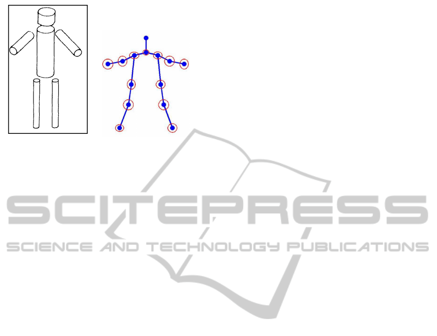
(a) (b)
Figure 1: Pose models in a still frame. (a) is the classic
articulated limb model of (Marr and Nishihara, 1978), (b) is
the model of (Yang and Ramanan, 2011).
body and a thigh are several examples of such parts.
Modern models defines a human pose in tersm of a
set of human body joints (fig. 1, b). A shoulder, a
knee and an elbow are some examples of such joints.
This definitions are equivalent. Indeed, the location of
each part is uniquely defined by locations of the cor-
responded joints, and a location of a joint is uniquely
defined by a location of the corresponded human body
part. In the research we exploit the second definition
as it makes the inference easier (Yang and Ramanan,
2011).
Most of the previous approaches to the human
pose estimation task work with still frames only. In
such case, the problem is usually reduced to infer-
ence in a tree structured graphical model. In this
models vertices correspond to locations of the joints
and edges define limitations on relative joint locations
(Yang and Ramanan, 2011). Due to the structure of
the graphical model the best configuration of a joint
location in a still frame can be obtained efficiently. In
spite of significant progress in techniques of the hu-
man pose estimation in a still frame, their accuracy is
far from ideal. Therefore we propose to improve the
accuracy of pose estimation by considering all video
frames simultaneously. The proposed approach uses
evidence of the pose from the other frames for the re-
sult gaining in the current frame. We use the tracking
approach (Shalnov and Konushin, 2013) to initially
estimate trajectory of the person. A trajectory means
an approximate location of the person in each frame
of the input video sequence. Hence, the formal input
of our algorithm consists of:
• video sequence W =
{
I
t
}
;
• trajectory of the person Ba =
{
B
t
}
.
The output of the algorithm is:
• human pose in the input video sequence. It means
location of joints and a scale parameter of the per-
son in each frame of the input video Pa =
{
P
t
}
.
2.2 Basic Model
Our research was inspired by the work of (Park and
Ramanan, 2011) on human pose estimation in video
sequence. They use the mathematical model of hu-
man pose in a still frame (Yang and Ramanan, 2011)
and expand the inference algorithm. Compared to
the previous method the extension by (Park and Ra-
manan, 2011) allows inference N-best configurations
from the model, ensuring that they do not overlap ac-
cording to some user-provided definition of overlap.
Moreover, they include a simple temporal context
from neighboring frames in the model. It allows them
to select better pose hypothesis in each frame of the
input video sequence. This way they converts the
problem of the human pose estimation in video to the
following maximization task:
Pa
∗
= argmax Score(Pa)
Score(Pa) =
∑
t
Φ(P
t
) + α
∑
t
Ψ(P
t
, P
t−1
)
(1)
where Φ(P
t
) is the score of candidate pose P
t
com-
puted by the proposed detector, and Ψ(P
t
, P
t−1
) is
the (negative of the) total squared pixel difference be-
tween each joint in pose P
t−1
and pose P
t
.
A set of available inference algorithms is the key
distinction between human pose models in still frame
and in video. A dynamic programming algorithm is
usually applied to infer optimal pose in a still frame.
However, it cannot be utilized to infer the optimal set
of poses in video. Indeed, the poses in instant of time
t
1
and t
2
are conditionally independent given a pose
at instant of time t ∈ [t
1
,t
2
] at least. Therefore, in-
ference with the dynamic programming algorithm re-
quires O(L
2K
) elements stored in memory, where L is
a number of possible joint locations in the frame and
K is a number of joints in the model. The authors use
an approximate algorithm. They restrict the possible
poses in each frame with best hypotheses. It makes
the dynamic programming tractable.
2.3 Proposed Model
We use the same model of human pose in a still frame
of (Yang and Ramanan, 2011), but with different tem-
poral context. The temporal context of the original
model requires the shift of joint location between sub-
sequent frames to be small. In practice, this constraint
is a poor motion model for a majority of body joints.
For example, the Brownian movement and the con-
stant motion with the same velocity have equal impact
to the objective function.
IMTA-52015-5thInternationalWorkshoponImageMining.TheoryandApplications
72

Therefore, we propose to use another temporal
context. Our temporal context prefers constant mo-
tion of the joints. We are aware of the model doesn’t
fully corresponds to the joint motion models observed
in practice. For example, a knee has a periodical mo-
tion model during walking. This periodicity is spec-
ified by the a cyclicity of a step. We choose the pro-
posed model as a simple and sufficient approximation.
We add velocity parameters for each joint to the
pose model to formulate the proposed motion model.
Therefore, the human pose P in a still frame I is de-
fined by the human scale parameter S and the joint
parameters

J
k

K
k=1
. The latter parameters include
joint locations Pos
k
and velocities V
k
in the follow-
ing form:
P = S ∪
n
J
k
o
K
k=1
J
k
=

Pos
k
,V
k

The objective function is similar to the one uti-
lized by (Park and Ramanan, 2011):
Score(Pa) =
∑
t
Φ(P
t
) +
∑
t
Ψ(P
t
, P
t−1
)
The temporal context is divided into two compo-
nents:
Ψ(P
t
, P
t−1
) = ψ
s
(S
t−1
, S
t
) +
K
∑
k=1
ψ
j
(J
j
t
, J
j
t−1
, S
t−1
)
The first component prefers the pose to have the
same size in all frames of the input video sequence:
ψ
s
(S
t−1
, S
t
) = −
1
2

S
t
− S
t−1
S
t−1
σ
s

2
And the second component has a form of a Linear
Dynamical System:
ψ
j
(P
j
t
, P
j
t−1
, S
t−1
) = −
dP
j
t
T
Σ
−1
p
dP
j
t
2S
2
t−1
dP
j
t
= (P
j
t
− AP
j
t−1
)
A =



1 0 1 0
0 1 0 1
0 0 1 0
0 0 0 1



Σ
p
=

Σ
p
p
Θ
Θ Σ
v
p

Σ
p
p
= α
−1
p
I
2×2
Σ
v
p
= α
−1
v
I
2×2
The proposed model corresponds to the constant
motion model with presence of normally distributed
error.
We want to notice that if the person scale parame-
ter does not change in the video sequence (S
1
= S
2
=
··· = S
N
= S), the basic model (Park and Ramanan,
2011) is a particular case of ours with the following
parameters:
α
p
= 2αS
α
v
→ inf
2.4 Inference Algorithm
The proposed modification of the pose model makes
dynamic programming unsutable for inference in
such model. The main reason for this is a dependence
of the velocity values on joint locations in all frames
of the video sequence.
Therefore, we use a MCMC sampling technique
to estimate the optimal value of the proposed score
function. We sample a set of hypotheses from the dis-
tribution p(Pa|W ) ∝ exp(Score(Pa)) to estimate the
optimal set of poses in the input video sequence. We
use the Metropolis-Hastings algorithm for sampling
(alg. 1). The sample with the highest score is cho-
sen as an approximation of the optimal solution. We
want to notice that the algorithm requires a transi-
tion model p(Pa
0
|Pa
l−1
) to sample from the specified
distribution. It defines the way of construction new
hypothesis Pa
0
from the previous one Pa
l−1
. An ac-
ceptance probability of the constructed hypothesis is
computed in the following way:
Acc(Pa
0
|Pa
l−1
) = min

p(Pa
0
|W )p(Pa
l−1
|Pa
0
)
p(Pa
l−1
|W )p(Pa
0
|Pa
l−1
)
, 1

It is important to notice that the Metropolis–
Hastings sampling algorithm imposes insignificant
limitations to a form of the optimized function. The
only limitation is an existence of the partition function
of the distribution p(Pa|W ). Therefore the proposed
pose model in a video sequence can be extended with
such global attributes of the observed human as a
color of clothes and a physique.
2.4.1 Transition Model
The sampling algorithm requires the transition model
p(Pa
0
|Pa
l−1
) to sample from the specified distribu-
tion. All of the proposed steps of the transition model
change only the pose joints locations and the scale pa-
rameters. Given the joint’s locations we can optimally
select hidden state values, as will be described in the
next section.
In our experiments we use several types of steps
to construct a new hypothesis of a set of human poses
in the video sequence:
HumanPoseEstimationinVideoviaMCMCSampling
73

Algorithm 1: An approximate algorithm of the hu-
man pose estimation.
Data: W, D
Result: Pa
Pa
0
= {argmax
P
t
p(P
t
|I
t
)}
N
t=1
;
for l = 1 to L do
sample Pa
0
∼ p(Pa
0
|Pa
l−1
);
compute Acc(Pa
0
|Pa
l−1
);
sample t ∼ U (0, 1);
if t < Acc(Pa
0
|Pa
l−1
) then
Pa
l
= Pa
0
;
else
Pa
l
= Pa
l−1
;
end
end
Pa = argmax
l∈
{
1,2,...L
}
p(Pa
l
|W );
1. a random perturbation in human joint locations at
the instant of time t;
2. a propagation of the human pose from the instant
of time t − 1 to the next instant of time;
3. a linear interpolation of the human pose in the in-
terval [t
1
,t
2
];
4. a replacement of the pose at the instance of time t
by one of hypothesis constructed by the algorithm
of (Park and Ramanan, 2011).
All of the proposed steps require the time instance
t or the interval [t
1
,t
2
] to be chosen. We want to notice
that the choice of the interval is equivalent to choice
of two instants of time. To speedup convergence we
make the algorithm to prefer instances of time that
have smaller confidence of the pose estimation cor-
rectness:
ξ(t) = Φ(P
t
) +
1
2
(Ψ(P
t
, P
t−1
) + Ψ(P
t+1
, P
t
))
p(t) ∝ max
τ
ξ(τ) − ξ(t)
The first step type adds a small perturbations in
the human joint locations and scale parameter at the
instance of time t. This modification has the following
form:
Pos
j
t
0
= Pos
j
t
+ βS
t
;
S
t
0
= S
t
+ γ
β ∼ N(0, β
−1
p
I
2×2
)
γ ∼ N(0, γ
−1
p
)
(2)
The second step type modifies a human pose at the
instance of time t by the propagation of its pose from
the previous instance of time and addition a normally
distributed noise according to (2). It uses the motion
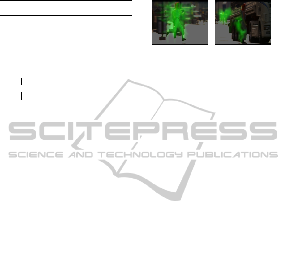
(a) (b)
Figure 2: Visualization of best constructed hypotheses.
Area, where most hypotheses were found, are highlighted
in green. In frame (a) detector find a lot of good hypotheses.
In frame (b) detector cannot find a good set of hypotheses.
parameters to construct more likely hypothesis. For
the first pose in the input video sequence this type of
steps is equal to the previous one.
The third step type modifies a set of the human
poses in the interval [t
1
,t
2
]. All poses inside the inter-
val are constructed by a linear interpolation between
the poses directly preceding and following the inter-
val.
The fourth step type exploits only a set of hypothe-
ses from the constructed by the human pose estima-
tion algorithm in the still frame. It replaces a pose
at instant of time t with one of hypotheses from the
constructed set. It prefers hypotheses that match the
proposed temporal context, i.e. minimize Ψ(P
t
, P
t−1
)
+ Ψ(P
t+1
, P
t
).
The fourth step type allows the inference algo-
rithm to use high-scored poses found in a still frame.
It speedups optimization in earlier stages. In figure 2
we demonstrate an area, where the best pose hypothe-
ses were found. In other hand, it makes the inference
sensitive to mistakes of human pose detector in a still
frame (fig. 2 b). Therefore, we add the first three
types of steps to deal with this problem.
2.4.2 Hidden State Estimation
As described above, the transition model modifies
only joint locations and the scale parameters. There-
fore the joint velocity values should be estimated. We
choose the optimal values of the velocity parameters
after each type of steps. In other words we chose val-
ues of the velocity parameters that maximize the score
function:
V
l
= argmax
V
Score(Pa)
Velocities of the different joints are independent
given the joint locations in the proposed model of the
human pose in a video. Consequently, the velocity
parameters of each joints can be estimated separately.
The form of the term ψ
j
(J
j
t
, J
j
t−1
, S
t−1
) implies
that the function Score(Pa) is factorized accordingly
to the graphical model presented in the figure 3 given
IMTA-52015-5thInternationalWorkshoponImageMining.TheoryandApplications
74

the human joint locations and the scale parameters.
Therefore the velocity of each joint can be estimated
efficiently.
We break the term φ
j
(J
j
t
, J
j
t−1
, S
t−1
) into unary and
pairwise terms based on the joint velocity parameters
(we skips parameters of the terms to simplify descrip-
tion):
ψ
j
= ψ
u
j
(V
j
t−1
) + ψ
p
j
(V
j
t−1
,V
j
t
)
The unary and the pairwise terms have the following
form:
ψ
u
j
(V
j
t−1
) = −
E
u
j
t
T
Σ
p
p
−1
E
u
j
t
2S
2
t−1
E
u
j
t
= ∆Pos
j
t−1
− A
u
V
j
t−1
∆Pos
j
t
= Pos
j
t
− A
u
p
Pos
j
t−1
ψ
p
j
= −
E
p
j
t
T
Σ
v
p
−1
E
p
j
t
2S
2
t−1
E
p
j
t
= V
j
t
− A
p
V
j
t−1
A =

A
u
p
A
u
Θ A
p

A
u
p
, A
u
, A
p
∈ R
2×2
In this form the problem of a posterior velocity es-
timation is equal to the inference problem in the fol-
lowing Linear Dynamical System:
V
j
= argmax
V
j
p

V
j
|∆Pos
j

∆Pos
j
t
∼ N(A
u
V
j
t
, Σ
p
p
)
V
j
t
∼ N(A
p
V
j
t−1
, Σ
v
p
)
V
j
1
∼ N(µ
0
, Σ
0
)
V
j
N
= A
p
V
j
N−1
µ
0
= Θ
2×1
Σ
0
= σ
0
I
2×2
σ
0
→ ∞
where ∆Pos
j
is a set of observed normalized velocity
values of the human joint, V
j
is a set of normalized
values of the hidden velocity parameters:
∆Pos
j
t
=
∆Pos
j
t
S
t
V
j
t
=
V
j
t
S
t
We use the Kalman filter with the RTS smoother
(Rauch et al., 1965) to estimate the optimal values of
the joint velocity.
We simulate a prior distribution on each compo-
nent of the velocity parameters in the first frame with
the normal distribution with dispersion going to infin-
Algorithm 2: An algorithm of a joint velocity V
j
es-
timation.
Data: ∆Pos
j
1
, . . . , ∆Pos
j
N−1
are the observed
data, (A
u
, A
p
, Σ
p
p
, Σ
v
p
) are the model
parameters
Result: µ
j
1
, . . . , µ
j
N
, Σ
j
1
, . . . , Σ
j
N
// the Kalman filter;
K
1
= A
uT

A
u
A
uT

−1
;
ˆµ
j
1
= K
1
∆
Pos
j
1
;
ˆ
Σ
j
1
=

A
uT
A
u

−1
A
uT
Σ
p
p

A
u
A
uT

−1
A
u
;
for t = 2,. . . , N-1 do
˜
Σ
t−1
= A
p
ˆ
Σ
j
t−1
A
pT
+ Σ
v
p
;
K
t
=
˜
Σ
t−1
A
uT
(A
u
˜
Σ
t−1
A
uT
+ Σ
p
p
)
−1
;
ˆµ
j
t
= A
p
ˆµ
j
t−1
+ K
t

∆Pos
j
t
− A
u
A
p
ˆµ
j
t−1

;
ˆ
Σ
j
t
= (I − K
t
A
u
)
˜
Σ
t−1
;
end
// The RTS smoother;
µ
j
N−1
= ˆµ
j
N−1
;
Σ
j
N−1
=
ˆ
Σ
j
N−1
;
for t = N-2,. . . ,1 do
K
t
=
ˆ
Σ
j
t
A
p
˜
Σ
−1
t
;
µ
j
t
= ˆµ
j
t
+ K
t
(µ
j
t+1
− A
p
ˆµ
j
t
);
Σ
j
t
=
ˆ
Σ
j
t
+ K
t
(Σ
j
t+1
−
˜
Σ
j
t
)K
T
t
;
end
µ
N
= A
p
µ
j
N−1
;
Σ
j
N
= Σ
v
p
+ A
p
Σ
j
N−1
A
pT
;
ity. Consequently, it indicates an absence of a prior
preferences on the velocity. It implies the following
modifications in the Kalman filter:
K
1
= A
uT

A
u
A
uT

−1
ˆµ
j
1
= K
1
∆Pos
j
1
ˆ
Σ
j
1
=

A
uT
A
u

−1
A
uT
Σ
p
p

A
u
A
uT

−1
A
u
We estimate the values of V
j
t
by the Viterbi algo-
rithm (Viterbi, 1967) for LDS (alg. 2). It means that
the original velocity parameters has the following es-
timations:
V
j
t
|∆
Pos
j
∼ N

S
t
µ
j
t
, S
2
t
Σ
j
t

3 RELATED WORKS
The mathematical model proposed in (Yang and Ra-
manan, 2011) is based on the deformable part model.
We use it as a basic model of a human pose in a still
frame.
HumanPoseEstimationinVideoviaMCMCSampling
75

P os
j
1
P os
j
2
P os
j
3
P os
j
N
S
1
S
2
S
3
V
j
1
V
j
2
V
j
3
V
j
N
Figure 3: A graphical model for a joint velocity estimation. Nodes of the observed variables are shown in gray.
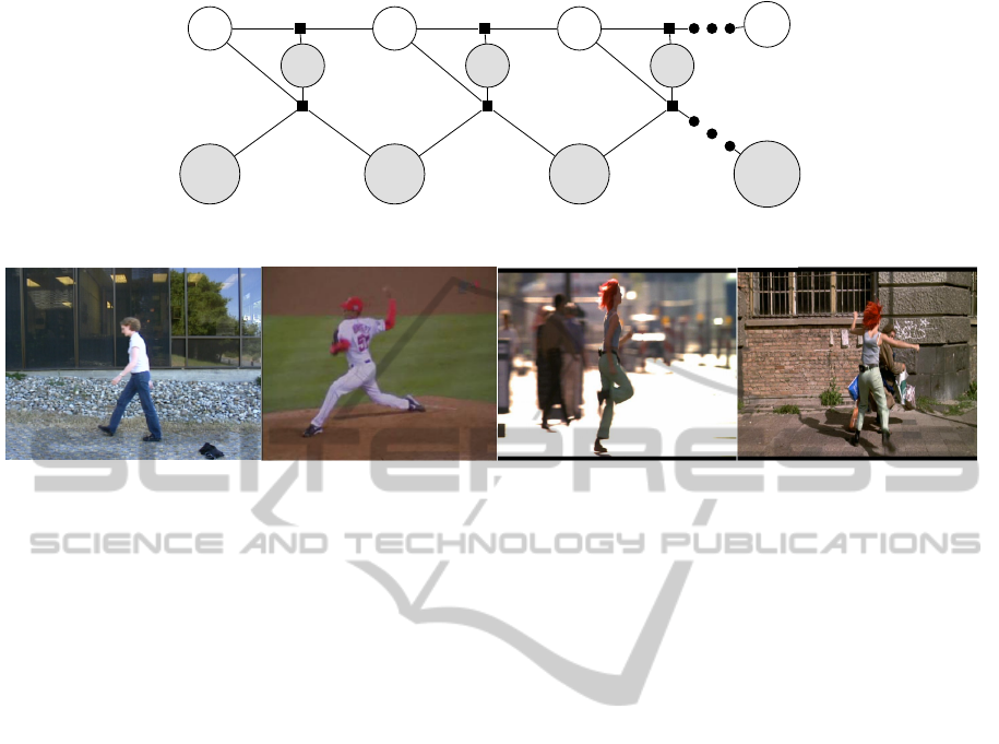
Figure 4: Frames from the dataset. From left to right, videos are called Walking, Pitching, Lola1, Lola2.
The deformable part model often fails in case of
occlusions. It localizes each joint of the person based
on evidence from the joint detector and location of
the neighbours. In case of occlisions the detector is
fully confident of the joint absence in its true position.
One feasible solution of this problem was proposed
in (Ghiasi et al., 2014). The authors extend number
of detectors associated with each joint with detectors
for occluded joints. The main disadvantage of this
approach is a necessity of a prior knowledge of occlu-
sion type. The authors consider only occlusions by
another person. This approach can be applied in our
framework in the future.
(Sapp et al., 2011) use the deformable part model
for the human pose estimation in a video as well. In
opposite to (Yang and Ramanan, 2011), they don’t
restrict the algorithm with sets of hypotheses con-
structed for each video frame separately. It makes the
inference task much more complicated. In particular,
they have to use an approximate inference algorithm.
Our algorithm of human pose estimation in a
video isn’t restricted to a choice from the set of hy-
potheses as well. The specific choice of the infer-
ence method was inspired by successful usage of the
sampling technique for the tracking task (Shalnov and
Konushin, 2013). In addition, it makes inference in
complicated mathematical models possible. It allows
further development of our model.
The deformable part model is not the only ap-
proach to human pose modeling. Recently the
convolutional neural networks (CNN) has become
widespread for image analysis. The authors of (To-
shev and Szegedy, 2013) propose a CNN model of
human pose in a still frame. The proposed algorithm
achieved the best results in the standard datasets. Un-
fortunately, we cannot apply this approach in our
model, because it doesn’t allow neither construction
of several hypotheses of a human pose, nor quality
estimation of the outside specified pose.
(Girshick et al., 2014) proposes a way to construct
an inference algorithm for the deformable part mod-
els as CNN. It makes possible to use an optimized
and fast developing software tools (Jia et al., 2014)
to human pose estimation task. In addition, it allows
an adjustment of parameters for both the deformable
part model and a feature extraction algorithm. We re-
gard this approach as a most promising for the future
development of the model.
4 EMPIRICAL EVALUATION
4.1 Setup
We quantitatively evaluate our algorithm on the pub-
licly available dataset (Yang and Ramanan, 2011).
Several frames from this dataset are shown in figure
4. The dataset includes 4 video sequences: Pitching,
Lola1, Lola2 and Walking. The videos are different
in complexity. The video sequences Pitching, Lola1
and Lola2 contain motion of a camera. A zooming is
presented in Pitching. Lola2 contains several people
in a scene.
IMTA-52015-5thInternationalWorkshoponImageMining.TheoryandApplications
76

(a) (b)
Figure 5: Pose as a set of sticks. (a) shows the groundtruth
pose, (b) groundtruth and found poses. The ground truth
pose is shown in blue. The green sticks are correctly local-
ized accordingly to the PCP criterion, while the red sticks
are considered as a false detections.
4.2 Results and Discussion
We evaluate the algorithm using the Percentage of
Correct Parts (PCP) criterion introduced in (Ferrari
et al., 2008). PCP criterion has a fundamental defect.
It interprets a pose as a set of sticks (fig. 5 a) and clas-
sifies localization correctness for each of them inde-
pendently. The stick is considered to be correctly lo-
calized if the normalized distance between found and
groundtruth locations of its edges are within the spec-
ified threshold. The stick size is used as a normaliza-
tion constant. Therefore, the same joint location can
be correct for one stick and incorrect for another stick
(fig. 5 b). However, PCP is the now-standard criterion
for the human pose estimation task and we use it for
evaluation.
For a fair evaluation we don’t use tracking in the
initialization stage. Therefore, the algorithm assumes
that the prior distribution of human location is uni-
form in a video frame. We don’t tune parameters
for each video separately, on the contrary we use the
same parameters for all videos. We presents results of
comparison in figure 1. As a baseline we we use the
method from (Park and Ramanan, 2011).
Table 1: We compare average PCP for the proposed method
and the basic one. Results of the basic method are given
from the (Park and Ramanan, 2011). Our approach out-
performs the basic method in the most difficult video se-
quences.
Algorithm walking pitching lola1 lola2
basic 0.950 0.797 0.670 0.500
our 0.950 0.762 0.695 0.545
Figure 6: The diagram shows an impact of the different
types of steps to the optimized score.
The proposed method outperforms the baseline
in the most complicated scenarios Lola1 and Lola2.
The algorithm solves the ambiguity in presence of the
several people in Lola2. It is achieved due to the in-
formation of the walking direction for the person of
interest.
Walking is the simplest video in the dataset. The
results of our algorithm and the basic one aren’t dif-
fer in it. It is caused by limitations of the used hu-
man pose model in a still frame (Yang and Ramanan,
2011).
Our algorithm shows lower value of PCP criteria
in the Pitching video sequence. The sophisticated
motion of the human in the video sequence is the main
reason of the algorithm failure.
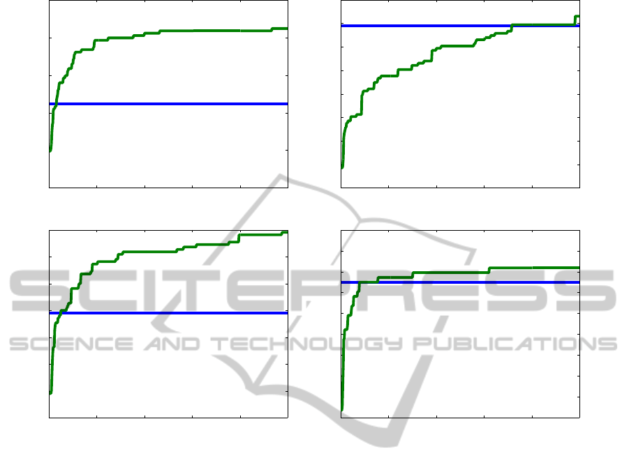
In addtion, we evaluate the upper bound of hu-
man pose estimation in a video in case of using only
hypotheses constructed by the detector of (Yang and
Ramanan, 2011). The results are shown in figure 7.
To evaluate the upper bound quality we construct a
set of best hypotheses as described in (Park and Ra-
manan, 2011) and choose the best one in each frame
using the PCP criterion.
The results show that our approach achieves al-
most optimal solution in lola1 and walking videos. in
pitching and lola2 videos our approach cannot come
near the optimal value. As we suppose the main rea-
son of such behaviour is a precense of nonlinear mo-
tions of limbs. walking and lola1 videos contain mo-
tion type that are more common in video surveillance.
4.3 Impact of the Different Steps
We evaluate an impact of different steps on the score
increase during the inference (fig. 6). The results
show that the second and the third types of steps pro-
duce the largest increase in the earlier stages of op-
HumanPoseEstimationinVideoviaMCMCSampling
77

0 100 200 300 400 500
0.65
0.7
0.75
0.8
0.85
0.9
N
Mean PCP
0 100 200 300 400 500
0.35
0.4
0.45
0.5
0.55
0.6
0.65
0.7
0.75
N
Mean PCP
pitching lola1
0 100 200 300 400 500
0.35
0.4
0.45
0.5
0.55
0.6
0.65
0.7
N
Mean PCP
0 100 200 300 400 500
0.82
0.84
0.86
0.88
0.9
0.92
0.94
0.96
0.98
1
N
Mean PCP
lola2 walking
Figure 7: We show the upper bound on the mean PCP value of hypotheses (green curve) as a function of number of hypotheses
(N). Our result values are shown as a blue line
timization. In the later stages the hypotheses con-
structed by those types of steps are rejected more fre-
quently by the sampling algorithm (alg. 1). Therefore
they bring the minor changes to the value of the opti-
mized function in the latter stages of optimization.
The first type of step increases score equally
throughout the optimization. But in each iteration
of the inference algorithm the increase is relatively
small.
5 CONCLUSIONS
In this paper we present the new mathematical model
of a human pose in a video sequence. Our model is
based on the model of human pose in a still frame
proposed in (Yang and Ramanan, 2011). We expand
this model with the new temporal context.
The proposed temporal context can be applied to
any model of human pose in a still frame that allows:
• estimation of an arbitrary pose quality in a frame;
• construction of most likely pose hypotheses in a
frame.
We show that the previous model (Park and Ra-
manan, 2011) is a particular case of the proposed one.
We propose the hidden state evaluation algorithm.
The proposed algorithm estimates the values of hid-
den state parameters given joint locations and scale
parameters.
We introduce a framework for a human pose esti-
mation in a video based on the MCMC sampling tech-
nique. The proposed algorithm allows furthur devel-
opment of our model with such global parameters of
the person as a physique and a color of clothes.
Our model and inference algorithm produce better
results in the most sophisticated videos of the dataset
in comparison with the basic algorithm (Park and Ra-
manan, 2011).
ACKNOWLEDGEMENTS
This publication is based on work funded by
IMTA-52015-5thInternationalWorkshoponImageMining.TheoryandApplications
78

Skolkovo Institute of Science and Technology
(Skoltech), contract #081-R, Appendix A 2.
REFERENCES
Ferrari, V., Marin-Jimenez, M., and Zisserman, A. (2008).
Progressive search space reduction for human pose es-
timation. In Computer Vision and Pattern Recogni-
tion, 2008. CVPR 2008. IEEE Conference on, pages
1–8. IEEE.
Ghiasi, G., Yang, Y., Ramanan, D., and Fowlkes, C. C.
(2014). Parsing occluded people. In Computer Vision
and Pattern Recognition (CVPR), 2014 IEEE Confer-
ence on, pages 2401–2408. IEEE.
Girshick, R., Iandola, F., Darrell, T., and Malik, J. (2014).
Deformable Part Models are Convolutional Neural
Networks.
Jia, Y., Shelhamer, E., Donahue, J., Karayev, S., Long, J.,
Girshick, R., Guadarrama, S., and Darrell, T. (2014).
Caffe: Convolutional architecture for fast feature em-
bedding. In Proceedings of the ACM International
Conference on Multimedia, pages 675–678. ACM.
Marr, D. and Nishihara, H. K. (1978). Representa-
tion and recognition of the spatial organization of
three-dimensional shapes. Proceedings of the Royal
Society of London. Series B. Biological Sciences,
200(1140):269–294.
Park, D. and Ramanan, D. (2011). N-best maximal decoders
for part models. Computer Vision (ICCV), 2011 IEEE
. . . .
Rauch, H. E., Striebel, C., and Tung, F. (1965). Maximum
likelihood estimates of linear dynamic systems. AIAA
journal, 3(8):1445–1450.
Sapp, B., Weiss, D., and Taskar, B. (2011). Parsing human
motion with stretchable models. In Computer Vision
and Pattern Recognition (CVPR), 2011 IEEE Confer-
ence on, pages 1281–1288. IEEE.
Shalnov, E. and Konushin, A. (2013). Improvement of
mcmc-based video tracking algorithm. In Pattern
rcognition and image analysis (PRIA-11-2013), pages
727–730.
Toshev, A. and Szegedy, C. (2013). Deeppose: Human pose
estimation via deep neural networks. arXiv preprint
arXiv:1312.4659.
Viterbi, A. J. (1967). Error bounds for convolutional
codes and an asymptotically optimum decoding al-
gorithm. Information Theory, IEEE Transactions on,
13(2):260–269.
Yang, Y. and Ramanan, D. (2011). Articulated pose estima-
tion with flexible mixtures-of-parts resenting shape.
2011 IEEE Conference on Computer Vision and Pat-
tern Recognition, pages 1385–1392.
HumanPoseEstimationinVideoviaMCMCSampling
79