
Seasonally Aware Routing for Thermoelectric Energy Harvesting
Wireless Sensor Networks
Aristotelis Kollias and Ioanis Nikolaidis
Computing Science Department, University of Alberta,Edmonton, T6G 2E8, Alberta, Canada
Keywords:
Thermoelectric Energy, Multi–commodity Routing, Energy–aware Routing.
Abstract:
Energy-aware routing schemes in wireless sensor networks (WSNs) often employ artificial energy assump-
tions, e.g., equal initial energy reserves for all nodes. Instead, we consider the case of realistic energy reserves
collected via thermoelectric energy harvesting in an apartment complex and examine how the harvested energy
impacts routing decisions over relatively large time frames. We formulate the corresponding multi-commodity
routing flow problem and, using real observed data, remark that maximizing the volume of collected data
typically leads to an uneven collection from each sensor. We propose a corresponding adjustment to the opti-
mization problem to derive a “fair” data collection strategy. We additionally present a low overhead method
of constructing a seasonally–aware routing scheme and study its performance. We compare the seasonally–
aware routing performance against that of an ideal, centralized, optimization solution, as well as against a
simple strategy to avoid extreme variance of residual energy at the sensor nodes.
1 INTRODUCTION
We consider the problem of multi-hop routing in
WSNs composed of nodes that exploit energy har-
vesting, and in particular energy harvesting through
the thermoelectric effect. Our objective is the multi-
decade autonomous operation of the WSN. The spe-
cific application domain considered is sensors embed-
ded in exterior walls in buildings, and more specif-
ically in Northern climates where, especially in the
colder months, the temperature difference between
indoor and outdoor provides abundant opportunities
for thermoelectric harvesting. In the networks con-
sidered, the topology is relatively static. The reasons
for embedding wireless rather than wired sensors is
primarily due the increased costs of wiring and labor
required to install such wiring. Moreover, the sensing
we would like to perform is generally taking place in
hard to reach locations, not necessarily conducive to
other forms of energy harvesting, e.g., photovoltaic
harvesting, due to lack of light and constraints stem-
ming from orientation/placement. On the contrary,
heat transfer is a universal phenomenon evidenced ev-
erywhere, albeit not always at levels that would pro-
vide for effective harvesting.
The results presented in this paper are based on
heat flow data collected at the exterior walls of an
apartment complex in (location redacted for double
blind review), Canada. So far, the data collected
were primarily used, by other works, for the purposes
of evaluating the building practices employed (in the
particular case, modular off-site construction accord-
ing to certain specifications) and the effectiveness of
using renewable resources like geothermal sources to
heating the building (Li et al., 2014; Sharmin et al.,
2014). We use the same data to determine what
would have been the data carrying capability if all lo-
cations where heat flow sensors were installed were
converted to wireless sensor nodes (compared to the
current, wired, albeit expensive, heat flow measure-
ments). Our intention is not to narrow the scope to
heat flow measurements alone, but, presented as a to-
tal volume of data, to allow the designer to decide
what data he/she would like to sample using in-wall
sensors. Of interest are, for example, the inclusion
of humidity measurements sensed within walls as in-
creased humidity is linked to both effects on the res-
idents (e.g., health effects from the growth of black
mold) and effects on the wall units (detrimental im-
pact to wall unit integrity and longevity).
We tacitly assume that all WSN nodes follow
a synchronized duty cycling scheme, whereby they
switch their transceivers ON once every time period
specified (typically once a day, unless otherwise in-
dicated) at which point the data transfers take place.
Data collection is assumed to be independently car-
174
Kollias A. and Nikolaidis I..
Seasonally Aware Routing for Thermoelectric Energy Harvesting Wireless Sensor Networks.
DOI: 10.5220/0005453601740184
In Proceedings of the 4th International Conference on Smart Cities and Green ICT Systems (SMARTGREENS-2015), pages 174-184
ISBN: 978-989-758-105-2
Copyright
c
2015 SCITEPRESS (Science and Technology Publications, Lda.)

ried out and data are accumulated at a sensor until
such time that they can be transmitted. We also as-
sume a static network topology with one node play-
ing the role of the sink. The single sink assumption
represents a worst case scenario inasmuch as it cre-
ates a focal point of congestion, but it is also the least
cost scenario (compared to multiple sinks) with re-
spect to installation cost. We assume the sink node
is not energy limited. Finally, we narrow our discus-
sion to the energy-related limitations of data transfers
and assume that wireless bandwidth is not a bottle-
neck, which is reasonable approximation of situations
where high data rates are possible and the volume of
data transferred are minuscule by comparison.
We model the problem as a multi-commodity
flow problem with each sensor’s data defining a sin-
gle splittable commodity routed through the network
topology but with different costs on the transmitting
and receiving side, to capture the general difference
of energy expenditure depending on whether a node is
transmitting or receiving. Our findings indicate that a
maximization of the total data volume collected at the
sink is generally an unfair solution in that not all sen-
sors are able to send the same amount of data to the
sink. We subsequently indicate that a constraint that
forces all sources to send the same total volume of
data to the sink, i.e., a concurrent multi-commodity
flow version, restores fairness, but we cannot avoid
the time-dependent nature of this fair share. Tech-
niques to mitigate this problem are discussed, and
in particular means to avoid extreme variance of the
residual energy of the nodes.
The next section, Section 2, summarizes related
work and places our contribution within the context
of this previous work. We provide the model for the
multi-commodity flow maximization and correspond-
ing routing in Section 3. Section 4 provides an eval-
uation of the multi-commodity formulation solutions
based on actual collected data. Section 5 introduces a
simple seasonally-aware routing scheme and remarks
on its efficiency. Section 6 provides some observa-
tions based on the evaluation results, and we conclude
with Section 7, which provides a summary of the pa-
per and future work directions.
2 RELATED WORK
Previous works, such as (Yerva et al., 2012), have as-
sumed that the energy harvesting nodes are the leaf
nodes of the network. Our work assumes that even
intermediary nodes are exploiting energy harvesting.
When a leaf node runs out of energy it impacts only its
own ability to collect and send data, but when an in-
terior node runs out of energy, it additionally impacts
routing. An interior node with limited energy harvest-
ing output, depending on its location to the overall
topology, can act as a bottleneck to the entire system.
In our study we essentially employ the interior nodes
in a balanced manner to maximize the ability to ac-
quire (or acquire in a fair manner) data from the entire
network.
Related to our approach is also (Sharma et al.,
2010) which describe means to maximize the
throughput but under the assumption of a single en-
ergy harvesting sensor observed in isolation. The gen-
eralization to the entire network we introduce in this
paper begs the question of whether the objective of
maximizing the throughput (i.e. sum–rate) or whether
maximizing a “fair” rate is more appropriate. We
adopt the convention that a fair allocation (same rate
of data delivery by each node in each “epoch”) corre-
sponds to the same sampling rate of the data at the
source, i.e., the fairness of transferred data volume
corresponds to fairness in terms of avoiding an un-
even sampling of the underlying phenomena across
different nodes.
Our work extends (and uses the same data set
as) our previous work (Kollias and Nikolaidis, 2014)
where we demonstrated that the difference in indoor
and outdoor temperature of apartments is a good
proxy for the heat flow measurements (to anticipate
the possibility that heat flow measurements are not
widely available) and hence as a proxy for the en-
ergy that can be harvested via thermoelectric mod-
ules. Specifically, by creating an experimental set-
ting to study the output of off–the–shelf thermoelec-
tric modules, we were able to derive an approximation
for the available thermoelectric energy, with the goal
of using the values to design an energy efficient sys-
tem. The details of how the energy is derived, are ex-
plained in (Kollias and Nikolaidis, 2014). We found
that there was ample energy to be harvested, but avail-
ability depends on the season and is highly variable,
when compared across apartments - ultimately linked
to the idiosyncratic behavior of the residents (what
thermostat set point they use, if they are present in
their apartments, etc.). The extension we consider in
this paper involves multi-hop routing and, hence, the
significant variability noted for individual nodes will
have an impact on the routing decisions.
In essence the problem we study involves the com-
bined effects of (a) the data collection as such and the
well-known fact that nodes closer to the sink are (de-
pleted of their energy first) as well as, (b), the effect
of the variable time-dependent behavior of the energy
harvested across different nodes. This is a significant
point of difference from previous, mostly abstract,
SeasonallyAwareRoutingforThermoelectricEnergyHarvestingWirelessSensorNetworks
175

work carried out in energy efficient routing (Singh
et al., 1998; Li et al., 2013) in that not all nodes start
with the same energy reserves or are able to replenish
to the same level their energy reserves.
The per-cycle operation we propose has strong
similarities to (Sadagopan and Krishnamachari, 2005)
in that, given the energy budget (or predictions there-
off) a multi-commodity flow problem needs to be
solved, but we additionally introduce the case of
fair–across–sources sensing. Moreover, the attention
of (Sadagopan and Krishnamachari, 2005) revolves
around the distributed implementation of the algo-
rithm which we forego for two reasons: (a) as in al-
most all WSN research, a supporting infrastructure is
assumed, such as a capable sink and/or an additional
backbone of computation resources outside the WSN
– we use this infrastructure to solve the flow problems
we have formulated and, (b), rather than spend energy
sending extra control messages between nodes in the
interest of an iterative distributed solution (shown in
(Sadagopan and Krishnamachari, 2005) to be O(N
4
)
or worse), we send a short status update (and new en-
ergy level) message from each node to the sink (typi-
cally requiring O(N
2
) messages), thus simplifying the
communication needs and leaving to the sink the bur-
den of the computational problem (in our case, the
solution of a, possibly large, LP).
Finally, in a particularly interesting variation of
the problem, reported in (Mara
ˇ
sevi
´
c et al., 2014),
multi-commodity flow has been used to show the
complexity of off-line instances of the fairness prob-
lem expressed across time (across “epochs”). Con-
trary to (Mara
ˇ
sevi
´
c et al., 2014), which currently
serves as a post-facto analysis of what could have
been the ideal forwarding, we use a multi-commodity
model to determine routing over each separate duty
cycle / epoch. In this sense, we are adopting the prob-
lem to a more realistic and practical setting whereby,
at each cycle, (new) decisions need to be taken on how
to forward the data to achieve throughput or fairness
objectives.
3 THE MODEL
Each sensor collects data independently of the rest.
The data of each node are treated as a separate com-
modity. The goal of every node is to send as much
data as possible with its current energy to the sink
using, possibly, multiple paths. Instead of stipulat-
ing which paths are to be used and which ones are
not, we pose the question as determining what frac-
tion of traffic for each commodity should flow across
each link with the purpose of either maximizing the
total, or, (in the second version) the total concurrent
volume of data delivered to the sink. By adopting a
multi-commodity model, we do not force a particular
routing, but rather we anticipate to observe that in op-
timal routing, when flows are split to traverse multiple
paths, such splitting will exhibit seasonal characteris-
tics, i.e., a particular link will be used certain times of
the year and not at others.
3.1 Maximum Multi-commodity Flow
Model
We consider the following multi–commodity maxi-
mization formulation of the routing problem on the
n sensor nodes (with t denoting the sink):
max
n
∑
i=1
( f
i
(s
i
,t)) (1)
s. t.
f
i
(s
i
,t) =
∑
w∈N
s
i
f
i
(s
i
,w) =
∑
w∈N
t
f
i
(w,t)
(2)
∑
w∈N
u
f
i
(u,w) =
∑
v∈N
u
f
i
(v,u)
(3)
q
n
∑
i=1
∑
v∈N
u
f
i
(u,v)
!
+ p
n
∑
i=1
∑
w∈N
u
f
i
(w,u)
!
≤ c(u)
(4)
Where f
i
(v,w) is the flow of commodity i from
node v to node w. Exceptionally, the auxiliary nota-
tion f
i
(s
i
,t) indicates the total flow from the origin of
commodity i (node s
i
) towards the sink t over possibly
multiple hops and paths. N
u
indicates the neighboring
(adjacent) nodes to node u. We assume the number of
nodes, minus the sink, is n. Equation 2 applies to all
commodities i and indicates that the total flow out of
the source and into the sink must be the same and is
equal to f
i
(s
i
,t). Equation 3 holds for each node u
(other than the sink) and commodity i and represents
the flow balance equation into and out of node u. Fi-
nally, equation 4 represents the constraint that the en-
ergy expended at node u cannot be more than c(u) (the
available energy). Here, q and p represent the ratios
of energy spent per unit of flow for transmitting and
receiving respectively.
By solving the above problem to determine
f
i
(v,w) in each duty cycle, using a linear program-
ming solver, we derive the maximum amount of data
that can be sent with the current energy levels in the
network. Using the computed solution, we can deter-
mine how much energy each sensor has to spend. We
SMARTGREENS2015-4thInternationalConferenceonSmartCitiesandGreenICTSystems
176

8
11
5
2
6
1
3
4
7
10
9
4th
3rd
2nd
1st
Figure 1: The network topology across building floors.
subtract that from the current energy of the nodes and
then we move to the next cycle, where the amount of
energy harvested is added to each node, and the multi-
commodity flow is solved again.
3.2 Maximum Concurrent
Multi-commodity Flow Model
Since the maximization of the total flow leads to ”un-
fair” results (explained in the next section), we also
consider a version whereby the objective is changed
to the following one:
max f
1
(s
1
,t) (5)
and we additionally introduce the constraint:
f
i
(s
i
,t) = f
1
(s
1
,t) ∀i (6)
The goal here is to maximize the flow as long as all
the commodities receive the same flow. Thus, the ad-
ditional constraint ensures that no commodity is going
to receive any worse service than any of the rest. Nev-
ertheless, we expect this to happen at the detriment of
the total flow. Furthermore, it should be clear that
solving the concurrent flow problem does not neces-
sarily result in the optimal use of the energy of the
nodes. In the concurrent version there will always
be sensors that have an excess of energy, which can
lead to many different maximum solutions, some of
them having wasteful energy expenditure, i.e., leav-
ing drastically different (and possibly low) residual
energy at the nodes. Consider the following example,
taken from our sample network in Figure 1, that illus-
trates the problem: Node 3 routes flow 3 to node 5.
Node 5 proceeds to route this flow to node 11 which
then routes it along the path to the sink. Node 5 also
routes flow 5 to node 3, which in turn routes it to node
1 to be routed along the path to the sink. If instead of
this, node 3 routed flow 3 to node 2, and node 5 routed
flow 5 to node 8, there would be less energy spent.
Nodes 11 and 1, which are closer to the sink, would
still need to route one complete commodity flow each,
which for them would cost the same, but node 5 and
3, instead of receiving one flow and sending two out,
will now just send one flow each. The reason that this
is allowed is that since the nodes 5 and 3 are closer to
the edges of the network, they have a lot more residual
energy, which allows them some flexibility on how to
spent their energy. The problem is that unnecessary
usage of energy like this, can lead to depletion of the
energy of those nodes in future cycles.
To address this shortcoming, we optimize with re-
spect to a secondary objective whose purpose is to
maximize the residual energy of nodes in anticipation
that it could be used in subsequent cycles. We remove
wasteful solutions produced by the maximum concur-
rent formulation, by creating a second LP problem
which, using the solution to the concurrent version
(let’s denote it by f
?
) explicitly minimizes the sum
across all nodes of the consumed energy, as captured
by equation 4. That is,
min
n
∑
u=1
q
n
∑
i=1
∑
v∈N
u
f
i
(u,v)
!
+
p
n
∑
i=1
∑
w∈N
u
f
i
(w,u)
!!
(7)
s. t.
f
?
= f
1
(s
1
,t) (8)
plus the additional constraints for flow conserva-
tion and source/sink flow summation we already pre-
sented. The reader should note however that this
minimization takes place over the sum of energy ex-
pended across all nodes, with no specific attention to
any single node.
A few technical remarks are in order: (a) we take
the approach that solving off-line the optimization
problem(s) and informing the nodes of the way to
route data is acceptable because the topology is static
and the information about the energy levels is rela-
tively short and could be communicated to the sink
(and from there to any optimization solution facility)
at the beginning of the duty cycle and the nodes can
be informed about the solution (delay is not a concern
as the operation of the network is duty cycled any-
way), and, (b) it is possible to generalize the fairness
captured by the concurrent formulation to a weighted
SeasonallyAwareRoutingforThermoelectricEnergyHarvestingWirelessSensorNetworks
177
fairness by setting f
i
(s
i
,t) = w
i
f
1
(s
1
,t) where w
i
’s are
fixed weights, in particular when it is known that cer-
tain nodes produce a constant factor more data than
others by virtue of the sensing they perform.
4 EVALUATION
In the evaluation section we assume that sensors at
the same floor and sensors on the same exterior wall
across adjacent floors are assumed to be within com-
munication range of each other.
We use data collected over the period from 25th
of June 2012 to 25th of June 2014. The structure of
our network is based on the structure of the apartment
building, that we have instrumented and from which
the measurements are collected. There are 4 floors in
the building, and 11 apartments are monitored. On
every floor except the bottom level there are 3 apart-
ments, two of which face South, while the third one
faces to the North. For our network we assume that
there is one node in each apartment attached to the
exterior wall, and each node can communicate with
all the nodes on the same floor, as well as with the
nodes at the same location on the floor plan on adja-
cent floors. The topology of the network (without the
sink) can be seen in Figure 1. We also consider two
different sink node placements: one at the fourth floor
and one at the second floor. A sink at a specific floor
can communicate in one hop with all the sensors at the
same floor. The reason for choosing these two floors
for the sink placement is to have a location close to
one extreme end of the building as well as one closer
to the “middle”.
For our experiments in this paper, q and p have
been chosen based on ratios characterizing actual RF
transceivers. In particular we adopt a model consis-
tent with the Silicon Labs Si106x (silabs.com, 2014).
The q/p ratios are: 1.31,2.12,5.11, 5.47,6.20. For
our duty-cycle, we have different timescales (per
hour, twice per day, per day, per week and per month),
which has given us a multitude of results. For this rea-
son, we choose in each figure to present the most in-
formative and general experiments, for each specific
situation.
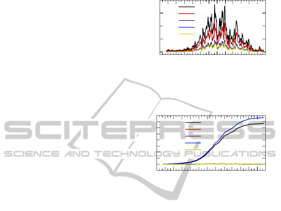
We started by trying to solve the routing using the
maximum multi-commodity flow model. Initially, we
assumed an unlimited energy storage capacity at the
nodes, for the purpose of seeing how the harvested en-
ergy scales across time. Results are shown in Figure
2. The results correspond to a daily duty cycling over
one year (starting on the 25th of June 2012 and end-
ing on the 25th of June 2013) and the solution of the
multi-commodity flow on a daily basis. After finding
0
5
10
15
20
06/01/2012
07/01/2012
08/01/2012
09/01/2012
10/01/2012
11/01/2012
12/01/2012
01/01/2013
02/01/2013
03/01/2013
04/01/2013
05/01/2013
06/01/2013
07/01/2013
1.31
2.12
5.11
5.47
6.20
10
2
J
Figure 2: Maximum multi-commodity flow solutions (daily
duty cycling, second floor sink, various q/p)).
-1
0
1
2
3
4
5
6
7
8
06/01/2012
07/01/2012
08/01/2012
09/01/2012
10/01/2012
11/01/2012
12/01/2012
01/01/2013
02/01/2013
03/01/2013
04/01/2013
05/01/2013
06/01/2013
07/01/2013
Node 1
Node 3
Node 5
Node 8
Node 10
10
4
J
Figure 3: Residual energy at certain nodes (second floor
sink, q/p = 1.31).
the solution for each flow, we subtract the energy used
from the energy already in the sensors. With this we
move to the next cycle, we add the new energy har-
vested and run the problem again. We can see how
the different q/p ratios bring different magnitude of
results. Clearly the range of values is vast. More in-
formative is Figure 3 which shows the residual energy
at the nodes on the daily timeframe if the duty cycling
was performed on a daily basis. We can see that the
nodes 3, 5 and 10, which are next to the sink and rep-
resent a bottleneck, are normally out of energy, while
all remaining sensors appear to have significant un-
used energy reserves. Indeed, if the objective is to
maximize the delivered data to the sink, regardless of
which sensor sends them, it is usually enough that all
the nodes near the sink spend all of their energy in
each cycle, trying to send only their commodity. This
leads to the maximum amount of data, since there is
no cost incurred by the sink’s neighbors for receiving,
consuming it exclusively to send data.
The apparent unfairness caused by maximizing
the delivered data is rectified by considering the con-
SMARTGREENS2015-4thInternationalConferenceonSmartCitiesandGreenICTSystems
178
0
5
10
15
20
06/01/2012
07/01/2012
08/01/2012
09/01/2012
10/01/2012
11/01/2012
12/01/2012
01/01/2013
02/01/2013
03/01/2013
04/01/2013
05/01/2013
06/01/2013
07/01/2013
Conc. max
Max
10
3
J
Figure 4: Comparison of maximum vs. concurrent maxi-
mum (q/p = 1.31).
current version of the multi-commodity flow problem.
In Figures 4 and 5 we can see the difference in results
between the maximum multi-commodity problem and
the maximum concurrent flow. For ease of compari-
son we have added all the flows in the concurrent flow
(essentially multiplying the flow by 11). We can see a
more significant difference when the ratio is smaller.
This happens because in both cases the sensors next to
the sink (there are three of them) are the bottleneck of
the routing. In the case of small q/p ratio, in the first
version of the multi-commodity problem they can just
use up all the energy transmitting, normalized by the
ratio to the sink, (energyo fthenode = datasent ∗ q)
while in the concurrent version the data that arrives
to the sink has a total cost to the three nodes around it
equal to (p+q)∗datasent ∗8/3+q ∗datasent (where
8 is the number of nodes that are not neighbors of the
sink, and hence rely on those neighbors for routing).
In the case of small ratio, q is smaller, therefore the
amount of data sent scales better for the first version.
Even though the maximum multi-commodity prob-
lem provides a better total throughput, the concurrent
flow is more useful due to the fact that the flows from
all nodes are equal, hence fair.
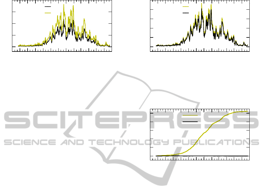
In the third set of experiments we limited the en-
ergy harvesting storage capacity. We assumed a su-
percapacitor of 5F and 5V that can store energy up to
62.5 Joules. The relevant results are shown in Fig-
ures 6 to 9. We compare the residual energy at certain
nodes, when the sink is on the second floor. It is ob-
vious that the capacitor adds a ceiling to the energy
gathered. We can see that when the duty cycling is
hourly, the limited capacity only affects the nodes far-
ther away from the sink, since those nodes generally
do not route much traffic through them, and since the
maximum amount of data they send is a small portion
to their overall energy levels, they tend to build up ex-
cess energy (only limited by the finite capacitor). A
0
10
20
30
40
50
06/01/2012
07/01/2012
08/01/2012
09/01/2012
10/01/2012
11/01/2012
12/01/2012
01/01/2013
02/01/2013
03/01/2013
04/01/2013
05/01/2013
06/01/2013
07/01/2013
Max
Conc. max
10J
Figure 5: Comparison of maximum vs. concurrent maxi-
mum (q/p = 5.11).
0
10
20
30
40
50
06/01/2012
07/01/2012
08/01/2012
09/01/2012
10/01/2012
11/01/2012
12/01/2012
01/01/2013
02/01/2013
03/01/2013
04/01/2013
05/01/2013
06/01/2013
07/01/2013
Unlimited
Limited
10
3
J
Figure 6: Energy at node 4 (1st floor) with and without lim-
ited capacity (the limited capacity line is imperceptible at,
almost, 0).
good example of this behavior is node 4 at the first
floor (Figure 6), which needs to transmit only its own
data, by virtue of being at the outskirts of the topol-
ogy, which means that it spends only a portion of the
energy other nodes spend – leading it to accumulate a
lot of energy over the course of a year.
Node 3, on the other hand, (Figure 7) is adjacent to
the sink, which leads it to use all of its energy in every
cycle. When the duty-cycle is per hour, we cannot
even notice a difference to the amount of energy the
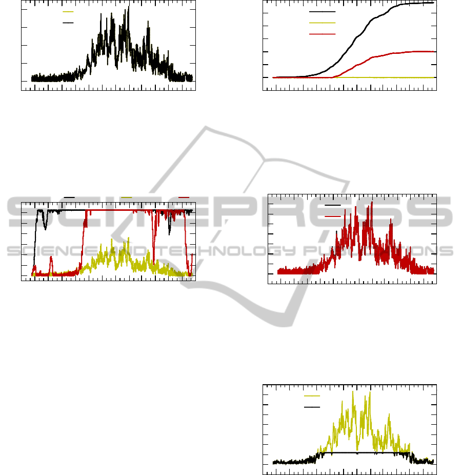
node has in the beginning of each cycle. In Figures
8 and 9 we can see how much the ceiling of limited
capacity affects the nodes that are not next to the sink.
Figures 10 and 11 demonstrate how the capacity
limit affects the results at hourly and twice per day
duty cycling. In Figure 10, the timescale is hourly and
the result of the multi-commodity routing does not
change significantly. This happens because the bottle-
neck sensors (adjacent to the sink) cannot gather en-
ergy fast enough to reach the capacity limit. It is more
interesting to see what happens when the timeframe is
SeasonallyAwareRoutingforThermoelectricEnergyHarvestingWirelessSensorNetworks
179
0
10
20
30
40
06/01/2012
07/01/2012
08/01/2012
09/01/2012
10/01/2012
11/01/2012
12/01/2012
01/01/2013
02/01/2013
03/01/2013
04/01/2013
05/01/2013
06/01/2013
07/01/2013
Unlimited
Limited
J
Figure 7: Energy at node 3 with and without limited capac-
ity (no evident difference).
0
10
20
30
40
50
60
70
06/01/2012
07/01/2012
08/01/2012
09/01/2012
10/01/2012
11/01/2012
12/01/2012
01/01/2013
02/01/2013
03/01/2013
04/01/2013
05/01/2013
06/01/2013
07/01/2013
Node 1 Node 10 Node 11
J
Figure 8: Energy at nodes 1, 10 (adjacent to sink), and 11
with limited capacity (node 10 is a bottleneck for routing).
twice per day (Figure 11). We can see that for most
part in the middle of the studied period (correspond-
ing to cold months where indoor/outdoor temperature
difference is significant, and hence harvesting is most
productive), there is a certain limit to what the sensors
can send. Ideally at that point we would use the ex-
cess energy for other functions, or even storing it to a
long term power storage like a battery (Rizzon et al.,
2013). However, what is noticeable overall from the
results so far, is that the extreme variance of energy
harvesting and usage at different times.
4.1 Dealing with Variability
In trying to solve the significant variance we wit-
nessed in empirical results, we imposed the ad-hoc
limit of using only 80% of the energy stipulated by
the flow problem solutions. That is, we reserve 20%
of each solution as backup that can then be part of
the residual energy surviving into the next cycle. The
simplicity of such a scheme was intentional, since one
could easily program such a “safety margin”. This led
-5
0
5
10
15
20
25
30
06/01/2012
07/01/2012
08/01/2012
09/01/2012
10/01/2012
11/01/2012
12/01/2012
01/01/2013
02/01/2013
03/01/2013
04/01/2013
05/01/2013
06/01/2013
07/01/2013
Node 1
Node 10
Node 11
10
3
J
Figure 9: Energy at nodes 1, 10, and 11 without limited
capacity (node 10 is the bottom line).
-0.5
0
0.5
1
1.5
2
2.5
3
3.5
4
06/01/2012
07/01/2012
08/01/2012
09/01/2012
10/01/2012
11/01/2012
12/01/2012
01/01/2013
02/01/2013
03/01/2013
04/01/2013
05/01/2013
06/01/2013
07/01/2013
Unlimited
Limited
J
Figure 10: Hourly duty cycling with and without capacity
limit (second floor sink).
0
5
10
15
20
25
30
35
40
06/01/2012
07/01/2012
08/01/2012
09/01/2012
10/01/2012
11/01/2012
12/01/2012
01/01/2013
02/01/2013
03/01/2013
04/01/2013
05/01/2013
06/01/2013
07/01/2013
Unlimited
Limited
J
Figure 11: Flow difference with and without capacity limit
(q/p = 2.11, twice per day duty cycling, fourth floor sink).
to some interesting results, which can be seen in Fig-
ure 12. The amount of data sent was very similar, as a
whole, to the standard concurrent maximum problem
– Figure 13 shows the results for duty cycling twice
per day (every 12 hours). The 20% reserve means that
there are not really completely depleted sensors in this
SMARTGREENS2015-4thInternationalConferenceonSmartCitiesandGreenICTSystems
180
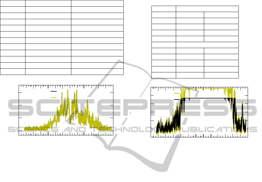
Table 1: Residual energy at nodes adjacent to the sink with
and without the 20% reserve (twice per day duty cycle).
node 3 w/ reserve node 3 w/out reserve
Average 46.58J 44.18J
Std Dev. 20.23 22.21
Min 7.55J 3.37J
node 5 w/ reserve node 5 w/out reserve
Average 50.69J 48.81J
Std Dev. 17.96 19.58
Min 5.02J 2.35J
node 10 w/ reserve node 10 w/out reserve
Average 44.44J 42.02J
Std Dev. 21.84 23.33
Min 4.97J 2.56J
0
0.5
1
1.5
06/01/2012
07/01/2012
08/01/2012
09/01/2012
10/01/2012
11/01/2012
12/01/2012
01/01/2013
02/01/2013
03/01/2013
04/01/2013
05/01/2013
06/01/2013
07/01/2013
no reserve
reserve
J
Figure 12: Hourly duty cycle, q/p = 5.11, with and without
20% reserve, sink at the fourth floor.
case.
Tables 1 and 2 present data about what happens
when we use the 20% reserve. In table 2 we can see
that the flows in the system do not really change if we
impose reserve if the duty cycling is on an hourly ba-
sis. The “bad days” continue to be very bad and the
“good days” do not change towards the better. When
the duty cycle is twice per day we find bigger dif-
ferences, as is also shown in Figure 13 – the flows
are slightly less than without the 20% reserve, which
is the case because for a significant part of the year
the capacity of the network is reached on every duty
cycle. The interesting part is that the standard devi-
ation is less, which means the network behavior is
more predictable, but even more importantly we can
see that the minimum flow is proportionally bigger
than the one without the 20% reserve. This can be
explained by the data in Table 1, where we can see
the residual energy for the three nodes adjacent to the
sink: on average they hold more energy in storage and
the minimum energy left on them in the beginning of
a duty cycle is significantly larger. It is this behavior
that provides more consistency to the network, allow-
ing for less chances that the nodes are depleted.
Table 2: Results for the concurrent maximum with and
without the 20% reserve (hourly and twice per day duty cy-
cle).
Hourly
w/ reserve w/out reserve
Average 0.79J 0.79J
Std Dev. 0.760 0.761
Min 0.0009J 0.0001J
Max 3.59J 3.60J
Twice/day
w/ reserve w/out reserve
Average 3.45J 4.09J
Std Dev. 1.643 2.20
Min 0.502J 0.306J
Max 4.79J 5.99J
0
5
10
15
20
25
30
06/01/2012
07/01/2012
08/01/2012
09/01/2012
10/01/2012
11/01/2012
12/01/2012
01/01/2013
02/01/2013
03/01/2013
04/01/2013
05/01/2013
06/01/2013
07/01/2013
no reserve
reserve
J
Figure 13: Twice daily duty cycle, with limited capacity,
q/p = 5.11, sink at the second floor.
5 A SEASONAL ROUTING
ALGORITHM
Until this point we have been examining the potential
of a centralized optimization execution to inform the
nodes as to their routing decisions. We remark now
on a strategy whereby the routing can be guided by
purely seasonal adjustments, independently by each
node without the continuous assistance of an opti-
mization to be run on the side. As stated in the work
where we first commented on the collected data (Kol-
lias and Nikolaidis, 2014), thermoelectric energy har-
vesting follows a strongly seasonal pattern. We tried
to take advantage of this quality of the data, by cre-
ating a very low overhead seasonal routing scheme.
The idea here is that we ”train” the sensors by us-
ing the data of the previous year(s), so that they can
be prepared for the second year. The process can
be extended to multiple years. In essence the multi-
commodity flow problem is solved for the first year,
and with it we create simple lookup tables (to guide
routing) at the granularity of week or month that are
SeasonallyAwareRoutingforThermoelectricEnergyHarvestingWirelessSensorNetworks
181
downloaded to the sensors and based on which rout-
ing will be performed in the subsequent year(s).
In Figure 14 one can see an example of how a node
can split its flows based on specific needs. This exam-
ple has the sink at the second floor, so node 7 is 2 hops
away from it (flow to 10 and then to the sink). The
boxes on the figure represent how node 7 would split
the total outbound flow from itself to the nodes 1,10
and 11 on the monthly timescale. Even though the
shortest path to the sink lies with node 10 (See Figure
1) we can see that while node 7 sends the majority
of its flow every month to node 10, to be forwarded
straight to the sink, it also sends significant amounts
to nodes 11 and 1 which are on the same distance to
the sink as it is. This happens because node 10 does
not have enough energy to route all the flows that pass
through 7. For this reason the node sends some of the
flows to 1 and 11 to be forwarded to nodes 5 and 3,
who have some energy to spare, with an extra hop.
This leads to more expenditure of energy but ends up
with a greater amount of flow for the network.
0
0.1
0.2
0.3
0.4
0.5
0.6
0.7
0.8
0.9
07/01/2012
08/01/2012
09/01/2012
10/01/2012
11/01/2012
12/01/2012
01/01/2013
02/01/2013
03/01/2013
04/01/2013
05/01/2013
06/01/2013
node 10
node 1
node 11
Figure 14: The split of flows from sensor 7 on a monthly
basis to nodes 1, 10 (adjacent to the sink) and 11.
Our approach consists of the following: we run
the multi-commodity flow problem for our network
based on the energy harvesting data from the previous
year, for weekly and monthly timeframes, keeping a
record of the split of the flows from each sensor (e.g.
the previous example of node 7). Subsequently, in ev-
ery timeframe of the second year (our validation set)
each node splits its flow of data according to a lookup
table created by the solutions from the previous year.
In essence each node holds a table that directs it to
send data according to calendar information
1
. Addi-
tionally, for the amount of data that the node actually
sends, the decision is taken according to how much
concurrent flow the whole network can send, then re-
1
The rows are the different seasons (we considered
weeks and months as two alternatives), and the columns are
the neighboring sensors. Each entry in the table is a ratio
that expresses the fraction of the data the node has to send
to that particular neighbor.
0
0.5
1
1.5
2
2.5
3
3.5
4
4.5
5
06/01/2012
07/01/2012
08/01/2012
09/01/2012
10/01/2012
11/01/2012
12/01/2012
01/01/2013
02/01/2013
03/01/2013
04/01/2013
05/01/2013
06/01/2013
07/01/2013
Conc. Max
Seasonal
J
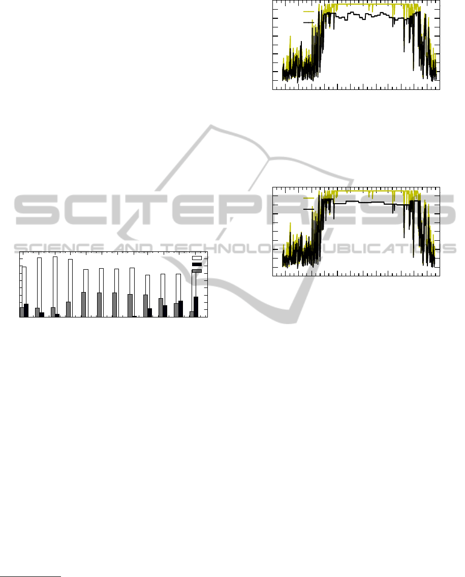
Figure 15: Twice per day duty cycling, weekly season,
q/p = 2.11.
0
0.5
1
1.5
2
2.5
3
3.5
4
4.5
5
06/01/2012
07/01/2012
08/01/2012
09/01/2012
10/01/2012
11/01/2012
12/01/2012
01/01/2013
02/01/2013
03/01/2013
04/01/2013
05/01/2013
06/01/2013
07/01/2013
Conc. Max
Seasonal
J
Figure 16: Twice per day duty cycling, monthly season,
q/p = 2.11.
duced by 20% reserve, for the same reason of reduc-
ing the impact of variability as shown earlier. Figures
15 and 16 show the results from seasonal aware rout-
ing (for q/p = 2.11) where the season is a week and a
month, respectively. The results are shown against the
corresponding hourly duty cycling (with 20% reserve)
concurrent maximum solutions. Our results indicate
that the seasonal aware routing was capable of routing
86.6% of the optimal flow allocation as would have
been determined by the concurrent maximum multi-
commodity flow over the same year. The percent-
age was not noticeably different regardless of whether
weekly or monthly season was used.
6 DISCUSSION
6.1 Maximum vs. Concurrent
Maximum
The solution to the multi-commodity problem we for-
SMARTGREENS2015-4thInternationalConferenceonSmartCitiesandGreenICTSystems
182

0
10
20
30
40
06/01/2012
07/01/2012
08/01/2012
09/01/2012
10/01/2012
11/01/2012
12/01/2012
01/01/2013
02/01/2013
03/01/2013
04/01/2013
05/01/2013
06/01/2013
07/01/2013
Node 2
Node 8
Node 11
10
2
J
Figure 17: Residual energy at nodes 2 and 8 (both adjacent
to the sink) and node 11 (3rd floor), with sink at the fourth
floor.
mulated has confirmed a well-known fact, that is,
that the biggest bottleneck is at the nodes adjacent to
the sink, as they are the ones who have to shoulder
the routing of all the data to their final destination. As
can be seen in Figure 9, other nodes might also strug-
gle in the beginning with initially small deposits of
energy, but after the winter season (where most har-
vesting happens) begins we can clearly see that the
sensors start accumulating significant energy deposits
(e.g., see nodes 11 and 1).
If the solution to the maximum concurrent multi-
commodity flow problem is to be used as the cen-
tralized routing scheme, it should be noted that the
sink should be placed at a location where its adjacent
nodes are the ones mostly benefiting from energy har-
vesting. In Figure 17 we can see that if the sink is
at the extreme side of the network (top floor of the
apartment building), nodes before that part can also
impose bottlenecks (here node 11 is the only node that
feeds node 8, which up to a point of the year does not
deplete its energy, because node 11 cannot forward
enough data to do so).
6.2 Infinite vs. Limited Capacity
In a realistic setting the nodes possess a finite energy
storage capacity, but as shown with Figure 6 they do
not really need it. The limited capacity impact de-
pends on the duty cycling period. If the duty cycle
is small enough (hourly in our case) it does not re-
sult in any significant difference, and as it increases,
changes become evident, especially in the high energy
availability seasons (Canadian winter). In Figure 11
we can see an actual difference for twice a day duty
cycling. There, fewer data are able to be transferred
to the sink from every node throughout most of the
winter period.
0
1
2
3
4
5
06/01/2012
07/01/2012
08/01/2012
09/01/2012
10/01/2012
11/01/2012
12/01/2012
01/01/2013
02/01/2013
03/01/2013
04/01/2013
05/01/2013
06/01/2013
07/01/2013
reserve
no reserve
10J
Figure 18: Node 2 with limited capacity, with and without
the 20% reserve.
6.3 20% Reserve and Limited Capacity
We tried to even out the variance of the flows across
different timeframes. Our solution to this was to engi-
neer a 20% reserve of the energy indicated by the con-
current maximum solution, thus ensuring that there is
always residual energy at all the nodes. Figure 18 il-
lustrates this technique by showing how much energy
exists in node 2 with and without the reserve. We can
see that in almost every cycle the node maintains more
energy in it, which results in the network being able
to route more flow per cycle, so in the end we do not
notice any significant difference in total flows routed
compared to not having a 20% reserve. However, if
nodes in the network reach the maximum capacity of-
ten, as in Figure 13, the scheme results in a decrease
of the total amount of data sent, because, systemati-
cally, 20% less data are being transferred.
6.4 Seasonal Routing vs. 20% Reserve
The idea of seasonally–aware routing is that in ev-
ery timeframe the node consults a lookup table to de-
termine what “season” it is in, and blindly sends the
data, spit accordingly, to the directions the table entry
points to. According to our experiments, (see Fig-
ure 15) this seasonal scheme, was successful at rout-
ing the 86% of the optimal concurrent maximum flow
even in the presence of a 20% reserve (to handle unan-
ticipated variability). Without being difficult to com-
pute and to install in the nodes, this routing scheme
seems very promising, and eliminates the need to de-
rive solutions to the multi–commodity flow problems
in every duty cycle.
SeasonallyAwareRoutingforThermoelectricEnergyHarvestingWirelessSensorNetworks
183

7 CONCLUSION AND FUTURE
WORK
In this paper we tried to model and solve the rout-
ing through an energy harvesting network, by formu-
lating multi-commodity flow problems. The multi-
commodity flow model can be used, along with its
slight variations, as a centralized routing scheme,
where the sink/central controller of the network de-
cides how the flow of data is going to be routed inside
the network, after getting all the information about
the residual energy at each of the nodes of the net-
work. We additionally proposed a distributed sea-
sonally aware scheme based on the concurrent multi-
commodity flow problem, which can run individually
at each node. All the techniques proposed, assume a
static network, where links between nodes are known
in advance.
For the future we would like to modify the multi-
commodity flow formulation so that it tries to op-
timize the residual energy in the nodes for use in
the next cycle, but with the added knowledge that it
distinguishes where this residual energy would bring
more benefit (i.e., at nodes adjacent to the sink). We
are currently working on prediction techniques for the
data, and in using adaptive duty cycling and energy-
neutral operation, from previous research works (Vig-
orito et al., 2007; Kansal et al., 2007), to achieve per-
petual operation of the nodes. Our primary goal now
is to implement a completely self–contained thermo-
electric harvesting node for in-wall use, using low
power microcontroller, and implementing these rout-
ing schemes with more realistic parameters (like the
inclusion of energy leakage etc.). Lastly we would
like to improve the seasonally aware routing scheme,
e.g., possibly by using machine learning techniques
and time series prediction models, to decide on the
split of flows and the amount of data sent, based on the
immediate neighborhood of the node (one hop away).
REFERENCES
Kansal, A., Hsu, J., Zahedi, S., and Srivastava, M. B.
(2007). Power management in energy harvesting sen-
sor networks. ACM Transactions on Embedded Com-
puting Systems (TECS), 6(4):32.
Kollias, A. and Nikolaidis, I. (2014). In-wall thermoelec-
tric harvesting for wireless sensor networks. In Pro-
ceedings of the 3rd International Conference on Smart
Grids and Green IT Systems, pages 213–221.
Li, W., Delicato, F. C., and Zomaya, A. Y. (2013).
Adaptive energy-efficient scheduling for hierarchical
wireless sensor networks. ACM Trans. Sen. Netw.,
9(3):33:133:34.
Li, X., Gul, M., Sharmin, T., Nikolaidis, I., and Al-Hussein,
M. (2014). A framework to monitor the integrated
multi-source space heating systems to improve the de-
sign of the control system. Energy and Buildings,
72(0):398 – 410.
Mara
ˇ
sevi
´
c, J., Stein, C., and Zussman, G. (2014). Max-min
fair rate allocation and routing in energy harvesting
networks: Algorithmic analysis. In Proceedings of the
15th ACM international symposium on Mobile ad hoc
networking and computing, pages 367–376. ACM.
Rizzon, L., Rossi, M., Passerone, R., and Brunelli, D.
(2013). Wireless sensor networks for environmental
monitoring powered by microprocessors heat dissipa-
tion. In Proceedings of the 1st International Work-
shop on Energy Neutral Sensing Systems, ENSSys
’13, page 8:18:6, New York, NY, USA. ACM.
Sadagopan, N. and Krishnamachari, B. (2005). Maximiz-
ing data extraction in energy-limited sensor networks.
International Journal of Distributed Sensor Networks,
1(1):123–147.
Sharma, V., Mukherji, U., Joseph, V., and Gupta, S.
(2010). Optimal energy management policies for en-
ergy harvesting sensor nodes. Wireless Communica-
tions, IEEE Transactions on, 9(4):1326–1336.
Sharmin, T., Gl, M., Li, X., Ganev, V., Nikolaidis, I.,
and Al-Hussein, M. (2014). Monitoring building en-
ergy consumption, thermal performance, and indoor
air quality in a cold climate region. Sustainable Cities
and Society, 13(0):57 – 68.
silabs.com (2014). Si106x-8x ultra-low power mcu with
integrated high-performance sub-1 ghz transceiver.
http://www.silabs.com/Support%20Documents/
TechnicalDocs/Si106x-8x.pdf. [Online; accessed July
2014].
Singh, S., Woo, M., and Raghavendra, C. S. (1998). Power-
aware routing in mobile ad hoc networks. In Proceed-
ings of the 4th annual ACM/IEEE international con-
ference on Mobile computing and networking, pages
181–190. ACM.
Vigorito, C. M., Ganesan, D., and Barto, A. G. (2007).
Adaptive control of duty cycling in energy-harvesting
wireless sensor networks. In Sensor, Mesh and Ad Hoc
Communications and Networks, 2007. SECON’07.
4th Annual IEEE Communications Society Confer-
ence on, pages 21–30. IEEE.
Yerva, L., Campbell, B., Bansal, A., Schmid, T., and Dutta,
P. (2012). Grafting energy-harvesting leaves onto the
sensornet tree. In Proceedings of the 11th interna-
tional conference on Information Processing in Sen-
sor Networks, pages 197–208. ACM.
SMARTGREENS2015-4thInternationalConferenceonSmartCitiesandGreenICTSystems
184
