Analyzing Multi-microgrid with Stochastic Uncertainties Including

Optimal PV Allocation

H. Keshtkar, J. Solanki and S. Khushalani Solanki

Department of Electrical Engineering, West Virginia University, PO Box 6070, Morgantown, WV 26505, U.S.A.

Keywords: PV Allocation, Loss Minimization, MATLAB-OpenDSS Interface, PSO, Multi-microgrid, Stochastic

Uncertainties, Stability Margin Analysis.

Abstract: This paper presents the effects of Photovoltaic (PV) location on losses of the distribution system. The optimal

location of PV is determined by using Particle Swarm Optimization (PSO) implemented in MATLAB-

OpenDSS environment. IEEE 34-node test feeder is employed to verify the feasibility and effectiveness of

the developed method. Once the optimal location is determined the challenge still remains due to the uncertain

behavior of the PV system. This effect along with other stochastic behaviors such as the uncertain output

power of loads like Plug-in Hybrid Electric Vehicles (PHEVs) due to their stochastic charging and

discharging, that of a wind generation unit due to the stochastic wind speed, and that of a solar generating

source due to the stochastic illumination intensity, add problems like frequency oscillations in a microgrid.

Hence, frequency control of a multi microgrid system is also addressed.

1 INTRODUCTION

Electric energy is produced in large power plants and

transmitted through High Voltage (HV) transmission

systems to be distributed to consumers through Low

Voltage (LV) distribution networks. Distribution

system dynamics are changing with the siting of

electricity generation closer to the loads and these are

called Distributed Generation (DG) units

(Mohammadi, 2012). These units have less

environmental impact, easy siting, high efficiency,

enhanced system reliability and security, improved

power quality, lower operating costs due to peak

shaving, and relieved transmission and distribution

congestion.

However, depending on the location of DG units,

some of the problems may be more pronounced and

hence it is important to site the DG units to optimally

exploit their potential. This paper, therefore, develops

algorithms to optimally place the distributed

generator considering the changing demand and

generation conditions over a day. With distributed

generators the distribution network can work in

isolation being separated from the feeder network to

form a micro-grid without affecting the transmission

grid’s integrity. One of the DG technologies is

Photovoltaic (PV), with penetrations increasing from

hundreds of kWs to MWs in LV network. Due to

these increasing penetrations in distribution systems,

the utilities and planning engineers are increasingly

interested in determining the best locations to place

these units (Prenc, 2013).

Much of the research work on PV allocation

assumes a constant generation making the problem

deterministic (Medina, 2006 – Shukla 2008). For

example, in (Shukla, 2008), analytical methods are

presented to determine the optimal location of PV

with constant generation to improve the power

quality. In reality however the PV output has

variations and hence an optimal location profiling the

daily irradiation and energy production is necessary

(Ackermann, 2001).

These units can be installed near load centers or at

remote nodes to avoid large power transfers. Since

distribution systems are now being operated as

microgrids that form smart cities, analysis on the

effects of these placements for microgrids is deemed

necessary (Duenas, 2014). The problem becomes

more complex with interconnection of multi-

MG/smart cities with more energy layers (Guo, 2010)

as compared to a single microgrid/smart city which is

a passive system.

In this paper we develop an optimal PV location

algorithm and analyze the effects of the PV

generations and loads like PHEVs on transient

stability of a multi-microgrid system. Since the

241

Keshtkar H., Solanki J. and Khushalani Solanki S..

Analyzing Multi-microgrid with Stochastic Uncertainties Including Optimal PV Allocation.

DOI: 10.5220/0005452902410249

In Proceedings of the 4th International Conference on Smart Cities and Green ICT Systems (SMARTGREENS-2015), pages 241-249

ISBN: 978-989-758-105-2

 2015 SCITEPRESS (Science and Technology Publications, Lda.)

variability of a PV system can affect the findings of

the optimal location a stochastic model is utilized for

both PV generations and PHEV loads. Stochastic

modeling and Monte Carlo simulation (MCS) are

common methods to perform the stochastic optimal

planning (Duenas, 2014), which have been widely

used in OPF (Guo, 2010, Zhang, 2011), distribution

network planning (Soroudi, 2011, Zhipeng, 2011),

power market design (Sofla, 2012 – Shresta, 2008),

distribution system extension planning (Kai, 2012)

and microgrid energy management (Niknam, 2012).

Here we utilize different models for stochastic

behaviors of variable generation and demand units.

The organization of this paper is as follows:

Section 2 discusses about modelling of the

distribution and microgrid system. The stochastic

modelling of uncertain parameters in the multi-

microgrid system is also formulated in this section.

PSO algorithm for optimal allocation of PV is

discussed in Section 3. Section 4 describes the case

studies and also presents the results of simulations.

The paper is concluded in Section 5.

2 MODELING AND PROBLEM

FORMULATION

We strongly encourage authors to use this document

several microgrids with many DG units such as

diesel, wind and solar generators integrated. In

distribution systems, losses can increase operation

cost and therefore it is essential to determine the

optimal placement of these generators to minimize

the total losses of the multi-microgrid system. Here

an optimal power flow type of problem is formulated

and heuristic algorithm such as particle swarm

optimization is selected.

2.1 Optimization Algorithm

In this paper we will consider the placement of solar

generation on ⊂ nodes of multi-microgrid due to

restriction imposed by distribution network operators.

We assume that solar generation contribute majorly

to the active power of the system thereby reducing the

problem to minimization of active power losses. The

methodology proposed here is described in three

basic steps:

1) A constrained non-linear optimization problem is

formulated to minimize the real power losses.

Equality constraints related to distribution power

flow equations and inequality constraints related to

node voltage limits, generation capacity constraints

and feeder current constraints are considered.

2) An intelligent computational technique like PSO

is employed with reduced computational complexity

due to reduction in search space from to 

where  are the number of PV units to be placed.

Since the order of units also matters a permutations

calculator rather than a combinations calculator is

employed.

3) PSO is combined with three phase distribution

power flow computed using backward forward sweep

algorithm while the PSO globally optimizes to find

the optimal DG placements and the distribution

power flow determines the constraints violations. In

backward forward sweep method, Kirchhoff’s

Current Law and Kirchhoff’s Voltage Law are used

to compute the bus voltage from farthest node in the

backward sweep. Then in forward sweep,

downstream bus voltage is updated starting from

source node. The procedure stops after the mismatch

of the calculated and the specified voltages at the

substation is less than a convergence tolerance.

4) If the optimal values of two consecutive iterations

are same with all constraints satisfied the algorithm is

deemed to have converged. If not, the process

continues until the criteria is satisfied.

The minimization objective function is formulated as

shown in (1).

loss







(1)

Considering the conductor current 



















∗

and

current contribution from the solar generator as



















∗

, the losses of line i

can be expressed as in (2).

3. .

cos sin

3. .

cos sin

ik ik

loss loss ik

iiii

kkkk

PIR





























(2)

The losses over a period of one day continuously

change due to changes in active power injections of

the solar generation and changes in load consumption

patterns. However, the location of PV once

determined cannot change, so an optimal location

should consider these variations in losses. The

optimization algorithm is subjected to the following

constraints.

(i) Generator Rating Constraint: Based on peak

power generation, the minimum and maximum

limits have been imposed on the generation

capacity as

SMARTGREENS2015-4thInternationalConferenceonSmartCitiesandGreenICTSystems

242

min max

iii

ggg

PPP

(3)

(ii) Voltage Constraint: The optimal siting has to

be obtained such that there are no bus voltages

limit violations.

min maxi

VVV

(4)

(iii) Power Balance Constraint: The total power

demand should be less than or equal to total

power generation.











(5)

(iv) Feeder Current Constraint: The feeder,

current flowing through the feeder should be

less than its thermal limit.

ik th

II

(6)

An unconstrained formulation considering both

objectives and constraints from (1-6) is then given in

(7). Typical operations constrain the voltage to be

around the nominal node voltages of the microgrid

whereas the lines have to be limited to their thermal

values.





11 1

()

ik i

NN r

xlossgd

ik i

Nom

gd ii

th ik

PPP

QQ VV

 







 

  







(7)

2.2 Power Flow Equations

The power balance constraints include the power flow

equations that are solved iteratively and expressed as

() () ()

ikk

Vi aV i bIi

icVidIi



(8)

Figure 1: Current flowing on line connecting node i and j.

The currents are those flowing on lines connecting

nodes i and j as shown in Fig. 1 and a,b,c,d are matrix

constants for the models of different components of

the distribution network. Here loads are modelled as

constant current injections,





















∗

, and

distributed generations as negative active power

loads. The generators are modelled using (9) that

relates the voltage

u and the current

NN N

ui s





(9)

where

s is the nominal complex power and



is a

characteristic parameter of the node N . The model (9)

is called exponential model (

Price, 1993) and is widely

adopted in the literature on power flow analysis

(Haque, 1996). Notice that

s is the complex power

that the node would inject into the grid, if the voltage

at its point of connection were the nominal voltage

U .

However, under islanded conditions the

microgrids lose stability instantly and hence

frequency response is of concern. The uncertain

behavior of the wind generations, hybrid electric

vehicles and solar generation result in frequency

deviations, an analysis of which requires uncertainty

models.

2.3 Uncertainty Models

The uncertainties considered in this paper include

wind speed, solar radiation, and load disturbance and

stochastic models for them are developed here:

2.3.1 Uncertainty of Wind Generating Units

It has been observed that wind speed deviations

follow a Weibull type distribution as shown in Eq.

(10) (Guo, 2010).

(,,) exp

kW W

pW ck

cc c





 





 



 



(10)

Where, scale factor 













and shape factor 











.

, W and σ are the average value and

standard deviations of wind speed, respectively, and

Γ(•) is the gamma function. Using the know

probability distribution function the relationship

between the output power of a wind generating unit

and the wind speed can be obtained and the details are

provided in (Mohammadi, 2012).

2.3.2 Uncertainty of Load

Load uncertainties are twofold: those associated with

AnalyzingMulti-microgridwithStochasticUncertaintiesIncludingOptimalPVAllocation

243

changing loads corresponding to daily consumption

and those corresponding to transportation related

consumption. For the daily consumption, hourly

average load demand is scaled by a disturbance factor

α=1+δ

, where δ

is the hourly disturbance coefficient

and α is the disturbance factor. Both α and δ

normal distribution with mean zero. Normal

distribution of load can perfectly model the variable

daily load in the power system P

=D*α is obtained

using D the hourly load data and α the disturbance

factor.

The other types of loads are the Plugin hybrid

electric vehicles. Since the behavior of consumers in

charging their PHEVs is highly behavior dependent,

three different stochastic processes for modelling

PHEV are considered here.

Brownian Motion: This is the continuous analog of

symmetric random walk distributions, where each

increment W(s+t)-W(s) is Gaussian with distribution

N (0, t) and increments over disjoint intervals are

independent. It is typically simulated as an

approximating random walk in discrete time. Here,

charging and discharging of PHEVs have been

modelled by Brownian motion with sigma of 3.

Poisson Process: This involves generation of random

events so that: (i) arrivals occur independent of each

other (ii) two or more arrivals do not occur at the same

time (iii) the arrivals occur with constant intensity.

Number of arrivals N (t) that occur from time zero up

to time t is Poisson distributed with expected value

lambda*t. The counting process N (t) is a Poisson

process. The successive times between connections

are Exponential (lambda) distribution. Here, arrival

time of PHEVs has been modeled by Poisson process

with lambda of 3.

M/M/1 Model: This is one of the random

distributions (Markov process) in the category of

Queuing systems. Discrete time intervals are

considered so PHEV arrivals to a service center occur

according to an independent sequence of a (1), a (2)

…, where a (k) is the number of arrivals during time

slot number k. Only one PHEV can be

charged/discharged per slot (single server system).

Additional PHEVs are in waiting until service is

available. Therefore the number of PHEVs in the

system at time k is given by



() ( 1) () 1, 2

(1)()1

(1) 0

nk nk ak k

nk ak

  

 



(11)

This recursion defines a Markov chain n (k), k ≥1. So

M/M/1 is a single server buffer model in continuous

time. Considering PHEV arrivals as Poisson process

with intensity λ, an exponentially distributed random

mean service time



 is employed for each PHEV.

The resulting system size N (t) for t ≥ 0, is a Markov

process in continuous time which evolves as follows:

Starting from N (0) = n_0, wait an exponential time

with intensity λ+μ (intensity λ if n_0=0), then charge

with probability /   and discharge with

probability /. Here, number of PHEVs in the

system (PHEV load size) has been modelled by

M/M/1 model with λ of 1.5 and μ of 0.8.

2.3.3 Uncertainty of PV

The uncertainty of solar radiation is mainly because

of the stochastic weather conditions. In this paper,

cleanness index is used to model the uncertainties of

weather condition. The relationship between the

cleanness index and the solar irradiation can be

obtained from (Srisaen, 2006). The distribution

function of cleanness index can be expressed as.

()

( ) exp( )

tu t

kC k







(12)

Where, k

indicates the mean value of cleanness

index, k

is the 0.864 theoretically, 



















where  2  17.519 exp



1.3118





1062exp



5.0426



/



and 



/









.

The PV generation varies with the solar

irradiation which varies according to the cleanness

distribution. The relationship between the solar

irradiation and the PV output power can be obtained

from (Huang, 2006).

2.3.4 Load Frequency Control (LFC)

Load Frequency Control (LFC) has been

implemented in the second part of the simulations for

a multi-microgrid system. LFC in microgrids with

nominal frequency of 50 Hz is designed to maintain

frequency within 49.9 and 50.1 in normal condition

by controlling tie-line flows and generator load

sharing (Kroposki, 2008). The control strategy should

damp the frequency oscillation in steady state and

minimize them in transient state while maintaining

stability.

Microgrids considered in this paper has hybrid

power generation consisting of wind generators,

photovoltaic, diesel generators. Power supplied to the

load Ps is the sum of output power from wind turbine

generators P

, diesel generators P

, photovoltaic

generation P

, total loss power P

Loss

and output of

PHEV P

phev

given by

wg pvlossphev

PPP P P



  

(13)

SMARTGREENS2015-4thInternationalConferenceonSmartCitiesandGreenICTSystems

244

Table 1: Total daily loss for different PV locations.

PV Bus 808 814 816 828 832 834 840 848 860 890

Total daily Loss (MWh) 3.8129 3.6524 3.6513 3.6182 3.4299 3.4457 3.4300 3.4294 3.4295 3.8688

LFC system in this paper uses this power flow

balance equation for adjusting the frequency of the

microgrid. Modeling of different parts of the system

is discussed in the rest of this section.

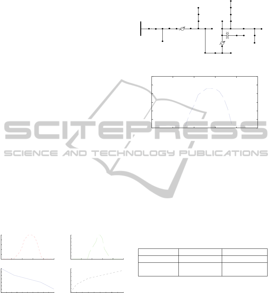
Modeling of Wind Turbine Generator (WTG). The

wind turbine is characterized by non-dimensional

curves of power coefficient C

as a function of both

tip speed ratio λ and blade pitch angle β. The tip speed

ratio, which is defined as the ratio of the speed at the

blade tip to the wind speed, can be expressed by

blade blade







(14)

Figure 2: Characteristic curve of output mechanical power

versus wind speed of the studied WTGs.

where R

blade

(= 23.5 m) is the radius of blades and

blade

(=3.14 rad/s) is the rotational speed of blades.

The expression for approximating C

as a function of

λ and β is given by

(3)

(0.44 0.0167 )sin 0.0184( 3)

15 0.3













  







(15)

The output mechanical power of the studied WTGs is

WrpW

AC V





(16)

where, ρ (= 1.25 kg/m3 ) is the air density and A

1735 m2) is the swept area of blades. The

characteristic curve of output mechanical power

versus wind speed of the studied WTGs in this paper

is shown in Fig. 2.

3 PARTICLE SWARM

OPTIMIZATION (PSO)

The locations of the PV systems are optimized by

Particle Swarm Optimization (PSO) Algorithm to

minimize the total losses in the system presented in

(7). PSO is a multi-agent search approach, which

traces its evolution to the motion of a flock of birds

searching for food. It uses a number of particles that

are called a swarm. Each particle traverses the search

space searching for the global minimum (or

maximum). In a PSO system, particles fly within a

multidimensional search space. During flight, each

particle sets its position based on its own experience

and the experience of neighboring particles. Hence, it

makes use of the best position encountered by itself

and its neighbors. Similarly, the swarm direction and

speed of a particle is determined by the history

experience obtained by itself as well as a set of its

neighboring particles (Babaei, 2009).

Each particle is a representative of PV locations

that are variables that affect the total losses in each

iteration. Let us consider p and s as particle position

and flight speed in a search space, respectively. The

best position of a particle in each step is recorded and

represented as P

best

. The best particle’s index among

all the particles in the group is considered as G

best

. The

convergence of PSO is ensured by use of a

constriction function. Finally, the modified velocity

and position of each particle can be calculated as

shown in (17) and (18):

11 2

*( * . ()*( ) * ()*( ))

dd bestd bestd

k v ac rand P P ac rand G P







 

(

17)

11ddd

PPs







(

18)

Here d is the index of iteration, P

is the current

particle’s position at the d-th iteration, s

is the

particle’s speed of at d-th iteration, γ is inertia weight

factor, ac

and ac

are acceleration constants, rand() is

a uniform random value in the range [0,1], and k is

the constriction factor which is a function of ac

and

according to (19):

|2 4 |

ac ac ac



 

(19)

Where ac=ac

+ac

and ac>4. Appropriate choice of

inertia weight, γ, makes a balance between global and

local explorations. In general, γ is calculated

according to (20) (Das, 2006):

max min

max

iter





 

(20)

AnalyzingMulti-microgridwithStochasticUncertaintiesIncludingOptimalPVAllocation

245

Where iter

max

is the maximum number of iterations,

and iter is the number of the iterations up to current

stage. The iterations continue until it reaches the

iter

max

or the difference between the losses calculated

by best particles of the last two iterations is less than

a predefined threshold.

4 CASE STUDIES AND

SIMULATION RESULTS

The optimal PV locations are determined using the

formulations discussed and the PSO technique. It is

shown that losses are minimized under varying daily

load consumptions. The PSO method described in

section 3 was implemented in Matlab programming

language and the unbalanced power flow solution is

obtained using OpenDSS. With the placement of PVs

at these optimal locations a frequency stability

analysis of a multi-microgrid system is performed

under stochastic load and generation behavior.

4.1 Optimal PV Allocation

As a preliminary analysis a 0.5 MW of PV generation

is considered with an unknown optimal location that

would result in minimum line losses. IEEE 34 node

benchmark distribution system as shown in Fig 4 is

considered that is inherently unbalanced with three

phase cables and conductors and three phase, two

phase and single phase loads. The characteristic

curves of the PV are as shown in Fig. 3 (a)-(d).

Figure 3: PV Characteristic curves; (a) Irradiation-time, (b)

Temperature-time, (c) P

mpp

-temperature, (d) Efficiency-

power.

Initially losses are evaluated with single PV

integration at node 848 of the IEEE 34 node system.

Losses for an entire day are plotted as shown in Fig.

5 as the PV generation and loads vary throughout the

day.

The active power losses are low at night and in

early morning time periods, when loading is less.

Figure 4: IEEE 34 node test feeder configuration.

Figure 5: Daily losses with PV placement at node 848.

However, when the loading increases and active

power generations from PV source increases, the

losses increase peaking from 15:00 – 16:00 hours.

Table 1 summarizes the total daily losses with PV

placements at different nodes. It is seen the best

location is node 848 which is located further from the

main grid and close to high-demand consumers.

Similar results are obtained using the developed PSO

algorithm and it is seen that losses are reduced by

29% as compared to no PV installation and 13% as

compared to worst PV installation.

Table 2: Total daily loss for best and worst multi-PV

locations.

Best PV locations Worst PV locations

PV Nodes 832, 848, 860 808, 814, 890

Total daily Loss

(MWh)

3.5620 3.8408

4.2 Optimal Multi-PV Allocation

Optimal locations for three PVs are obtained for IEEE

34 node test feeder by optimization algorithm (PSO)

to achieve the minimum total daily losses. As seen in

Table 2 the optimal node locations are 832, 848 and

860. They show 8% improvement in losses as

compared to the worst locations found heuristically.

4.3 Stochastic Uncertainties in

Multi-microgrid

With the determined optimal PV locations frequency

0 5 10 15 20 25

0.2

0.4

0.6

0.8

Time (hours)

Irradiation

(a) Irradiation-tim e

0 5 10 15 20 25

Time (hours)

Temperature

(b) Temperature-time

0 10 20 30 40 50 60 70 80 90 100

0.5

0.6

0.7

0.8

0.9

1.1

1.2

Temperature ('C)

Pmpp

0.1 0.2 0.3 0.4 0.5 0. 6 0.7 0. 8 0.9 1

0.86

0.88

0.9

0.92

0.94

0.96

0.98

Power (pu)

Efficiency

(d) Efficiency-output power

800

806 808

812

814

810

802

850

818

824

826

816

820

822

828 830

854 856

852

832

888

890

838

862

840

836860

834

842

844

846

848

864

858

0 5 10 15 20 25

0.16

0.17

0.18

0.19

0.2

0.21

0.22

Time (h)

Total Loss

Loss-time

SMARTGREENS2015-4thInternationalConferenceonSmartCitiesandGreenICTSystems

246

stability is evaluated considering the frequency

response models and uncertainty modelling in section

2. Moreover for multiple microgrids several islands

may occur simultaneously as a result of multiple

contingencies in the network. PSO is adopted here to

improve the frequency response by optimizing the

parameters of various controllers. The details of

controller design utilizing PSO for speed control are

available in our prior work (Keshtkar, 2014).

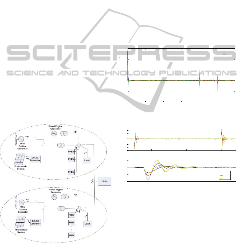
Consider two similar microgrids connected

through a tie line as shown in Fig. 6. This hybrid

system comprises of several RES such as Wind

Turbine Generator (WTG) and PV including Diesel

Engine Generator (DEG) as DG that contributes to

the inertia of the microgrid system. The hybrid system

also includes PHEVs and other residential and small

industrial loads. The PV systems are located

optimally using the algorithm proposed earlier in the

paper. The controllable source in this microgrid is

Diesel Engine Generator whose control parameters

are optimized by PSO to minimize the frequency

deviations due to the disturbances. The tie line

deviations of the multi-microgrid system are also

considered in the objective function for optimizing

controller parameters. The Area Control Error (ACE)

for each microgrid considering ΔP

tie

the tie-line

power flow deviation, Δf

the frequency deviation of

each microgrid weighted by β is as shown in (21).

i tie i

CE P f



  

(21)

Figure 6: Configuration of the modeled multi-microgrid.

Three different stochastic behaviors of the PHEVs

discussed in section 2 are modeled along with

stochastic uncertainties of load, wind and solar

generations. Frequency response of one of the

microgrids of the multi-microgrid system is obtained

as shown in Fig. 7. Also Fig. 8 shows the magnified

frequency responses of the system in presence of

different stochastic uncertainties in the multi-

microgrid power system.

It is seen that stochastic modeling is essential to

study the transient stability of the system and that

some uncertainties can cause the frequency to

severely deviate from the nominal value. For

example, stochastic behavior of PHEVs creates

significant overshoots in the frequency response as

shown in Fig. 8 that can cause the microgrid system

to be unstable. It is observed thus that a simultaneous

modeling of stochastic behaviors is essential to design

and test reliable and robust controllers.

Figure 7: Frequency response of one of the microgrids with

different stochastic modelling.

Figure 8: Frequency response of one of the microgrids for

stability margin analysis.

5 CONCLUSIONS

In this paper a method for determining the optimal

placement of a PV system in distribution network

based on daily power consumption/production

fluctuations is described to minimize the total daily

losses. The PSO optimization algorithm shows fast

and accurate performance in calculating the optimal

position of a PV system. Therefore, it can also serve

0 50 100 150 200 250 300

-0.01

-0.005

0.005

0.01

0.015

time

df-time

Brownian

Poisson

3D Brownian

M/G/Infinity

M/M/1

200 210 220 230 240 250

-8

-6

-4

-2

x 10

-3

time

(a) df-tim e

199 200 201 202 203 204 205

-8

-6

-4

-2

x 10

-3

time

(b) df-tim e

Brownian

Poisson

3D Brownian

M/ G/In finit y

M/M/1

AnalyzingMulti-microgridwithStochasticUncertaintiesIncludingOptimalPVAllocation

247

as a tool in calculating the optimal placement of any

number and kind of DG units with a specific daily

production curve such as wind turbine systems, fuel

cells, microturbines with a goal of optimizing

distribution power system performance.

A transient response analysis of the system with

optimal PV locations and stochastic modeling of

loads and generation is obtained and control

parameters are designed using PSO. It is observed

that simultaneous stochasticity modeling of all

components should be considered for designing

robust controllers.

ACKNOWLEDGEMENTS

The authors would like to acknowledge partial

funding support from NSF#1351201 CAREER grant

for this research work.

REFERENCES

Mohammadi M., Hosseinian S.H., and Gharehpetian G.B.,

2012. Optimization of Hybrid Solar Energy

Sources/Wind Turbine Systems Integrated to Utility

Grids as Microgrid (MG) Under Pool/Bilateral/Hybrid

Electricity Market Using PSO. Solar Energy, vol. 86,

pp. 112–125.

Prenc R., Škrlec D., Komen V. 2013. Optimal PV System

Placement in a Distribution Network on the Basis of

Daily Power Consumption and Production Fluctuation

EuroCon, Zagreb, Croatia.

Medina A., Hernandez J.C., and F. Jurado, 2006. Optimal

Placement and Sizing Procedure for PV Systems on

Radial Distribution Systems. International Conference

on Power System Technology.

Singh R. K., Goswami S. K. 2009. A Genetic Algorithm

Based Approach for Optimal Allocation of Distributed

Generations in Power Systems for Voltage Sensitive

Loads. ARPN Journal of Engineering and Applied

Sciences.

Prenc R., V. Komen, N. Bogunovi, 2012. GIS-based

Determination of Optimal Accommodation of

Embedded Generation on the MV Network.

International Journal of Communications Antenna and

Propagation.

Costa P. M., M. A. Matos, 2004. Loss Allocation in

Distribution Networks with Embedded Generation.

IEEE Transaction on Power System.

Srisaen N., and A. Sangswang, 2006. Effects of PV Grid-

Connected System Location on a Distribution System.

IEEE Asia Pacific Conference on Circuits and Systems.

Méndez V. H., J. Rivier, J. I. de la Fuente, T. Gómez, J.

Arceluz, J. Marín, 2002. Impact of Distributed

Generation on Distribution Losses. In Proc.

Mediterranean Power, Athens, Greece.

Shukla T.N., S.P. Singh and K.B. Naik, 2008. Allocation of

Optimal Distributed Generation using GA for

Minimum System Losses. Fifteenth National Power

Systems Conference (NPSC), IIT Bombay.

Ackermann T., G. Andersson, L. Söder, 2001. Distributed

generation: a definition. Electric Power Systems

Research, 2001.

Duenas P., Reneses J., Barquin J., 2014. Dealing with

multi-factor uncertainty in electricity markets by

combining Monte Carlo simulation with spatial

interpolation techniques. IET Gener. Transm. Distrib.

Guo L., Liu W., B. Jiao, B. Hong, C. Wang, 2010. Multi-

objective stochastic optimal planning method for stand-

alone microgrid system. IET Gener. Transm.

Distribution.

Zhang, H., Li, P., 2011. Chance constrained programming

for optimal power flow under uncertainty. IEEE Trans.

Power System.

Soroudi, A., Caire, R., Hadjsaid, N., Ehsan, M., 2011.

Probabilistic dynamic multi-objective model for

renewable and non-renewable distributed generation

planning. IET Gener. Transm. Distribution.

Zhipeng, L., Fushuan, W., Ledwich, G., 2011. Optimal

siting and sizing of distributed generators in distribution

systems considering uncertainties. IEEE Trans. Power

Delivery.

Sofla M. A., King R., 2012. Control Method for Multi-

Microgrid Systems in Smart Grid Environment -

Stability, Optimization and Smart Demand

participation. IEEE PES Innovative Smart Grid

Technologies (ISGT).

Shrestha, G.B., Pokharel, B.K., Lie, T.T., 2008.

Management of price uncertainty in short-term

generation planning. IET Gener. Transm. Distribution.

Kai Z., Agalgaonkar A.K., Muttaqi K.M., 2012.

Distribution system planning with incorporating DG

reactive capability and system uncertainties. IEEE

Trans. Sustain. Energy.

Niknam, T., Golestaneh F., Malekpour A., 2012.

Probabilistic energy and operation management of a

microgrid containing wind/photovoltaic/fuel cell

generation and energy storage devices based on point

estimate method and self-adaptive gravitational search

algorithm. Energy.

Price, W. W., Chiang, H. D., Clark, H. K., Concordia, C.,

Lee, D. C., Hsu, J. C., Vaahedi, E., 1993. Load

representation for dynamic performance analysis. IEEE

Transactions on Power Systems, 8(2), 472-482.

Haque M. H., 1996. Load flow solution of distribution

systems with voltage dependent load models. Elect.

Pow. Syst. Res., vol. 36, pp. 151–156.

Huang Y., Peng F.Z., Wang J., 2006. Z-Source Inverter for

Residential Photovoltaic Systems. IEEE Trans. Power

Delivery, vol.21, no.6.

Kroposki B., Basso T., and DeBlasio R., 2008. Microgrid

Standards and Technologies. IEEE Power and Energy

Society General Meeting, pp. 1-4.

Babaei E., Galvani S. and Ahmadi Jirdehi M., 2009. Design

of Robust Power System Stabilizer Based on PSO.

IEEE Symposium on Industrial Electronics and Appli-

SMARTGREENS2015-4thInternationalConferenceonSmartCitiesandGreenICTSystems

248

cations, Malaysia.

Das T.K., Venayagamoorthy G.K., 2006. Optimal Design

of Power System Stabilizers Using a Small Population

Based PSO. IEEE Power Engineering Society General

Meeting.

Keshtkar, H.; Mohammadi, F.D.; Ghorbani, J.; Solanki, J.;

Feliachi, A., 2014. Proposing an improved optimal

LQR controller for frequency regulation of a smart

microgrid in case of cyber intrusions. IEEE 27th

Canadian Conference on Electrical and Computer

Engineering (CCECE).

AnalyzingMulti-microgridwithStochasticUncertaintiesIncludingOptimalPVAllocation

249