Color Dog

Guiding the Global Illumination Estimation to Better Accuracy

Nikola Bani

c and Sven Lon

cari

Image Processing Group, Department of Electronic Systems and Information Processing,

Faculty of Electrical Engineering and Computing, University of Zagreb, 10000 Zagreb, Croatia

Keywords:

Clustering, Color Constancy, Illumination Estimation, Image Enhancement, White Balancing.

Abstract:

An important part of image enhancement is color constancy, which aims to make image colors invariant to illu-

mination. In this paper the Color Dog (CD), a new learning-based global color constancy method is proposed.

Instead of providing one, it corrects the other methods’ illumination estimations by reducing their scattering

in the chromaticity space by using a its previously learning partition. The proposed method outperforms all

other methods on most high-quality benchmark datasets. The results are presented and discussed.

1 INTRODUCTION

Color constancy is the ability to recognize object col-

ors regardless of the scene illumination (Ebner, 2007).

Achieving it is often used as a pre-processing method

in image processing because depending on scene il-

lumination, the image colors may differ as shown in

Fig. 1. Two steps are needed to achieve computational

color constancy: illumination estimation, the essen-

tial step, and chromatic adaptation using the estima-

tion, a relatively easy step. Both steps often use the

following image f formation model, which includes

Lambertian assumption:

(x) =

I(λ, x)R(x, λ)ρ

(λ)dλ (1)

where c is a color channel, x is a given image pixel,

λ is the wavelength of the light, ω is the visible spec-

trum, I(λ, x) is the spectral distribution of the light

source, R(x, λ) is the surface reﬂectance and ρ

(λ) is

the camera sensitivity of the c-th color channel. With

uniform illumination assumed, x is removed from

I(λ, x) and the observed color of the light source e

is:

e =









I(λ)ρ(λ)dλ. (2)

For successful chromatic adaptation only the

direction of e is important and its amplitude can be

disregarded. As it is often the case that the values

of I(λ) and ρ

(λ) are unknown, calculating e is an

(a) (b)

Figure 1: The same scene (a) with and (b) without illumi-

nation color cast.

ill-posed problem and additional assumptions are

taken to solve it. This has resulted in many color

constancy methods that form at least two groups.

The ﬁrst group is formed of low-level statistics-

based methods like White-patch (WP) (Land,

1977) and its improved version (Bani

c and

Lon

cari

c, 2014b), Gray-world (GW) (Buchs-

baum, 1980), Shades-of-Gray (SoG) (Finlayson

and Trezzi, 2004), Grey-Edge (1st and 2nd order

(GE1 and GE2)) (Van De Weijer et al., 2007a),

Weighted Gray-Edge (Gijsenij et al., 2012), us-

ing bright pixels (BP) (Joze et al., 2012), Color

Sparrow (CS) (Bani

c and Lon

cari

c, 2013), Color

Rabbit (CR) (Bani

c and Lon

cari

c, 2014a), using color

distribution (CD) (Cheng et al., 2014b). The second

group is formed of learning-based methods like

gamut mapping (pixel, edge, and intersection based -

PG, EG, and IG) (Finlayson et al., 2006), using

neural networks (Cardei et al., 2002), using high-

level visual information (HLVI) (Van De Weijer et al.,

2007b), natural image statistics (NIS) (Gijsenij and

Gevers, 2007), Bayesian learning (BL) (Gehler et al.,

129

Banic N. and Loncaric S..

Color Dog - Guiding the Global Illumination Estimation to Better Accuracy.

DOI: 10.5220/0005307401290135

In Proceedings of the 10th International Conference on Computer Vision Theory and Applications (VISAPP-2015), pages 129-135

ISBN: 978-989-758-089-5

 2015 SCITEPRESS (Science and Technology Publications, Lda.)

2008), spatio-spectral learning (maximum likelihood

estimate (SL) and with gen. prior (GP)) (Chakrabarti

et al., 2012), exemplar-based learning (EB) (Joze and

Drew, 2012), Color Cat (CC) (Bani

c and Lon

cari

2015). In devices with limited computation power

like digital cameras, faster low-level statistics-based

methods are used (Deng et al., 2011) because the

more accurate learning-based methods are slower.

Recently, a new learning-based method using the

illumination statistics has been proposed (Zhang and

Batur, 2014), which limits the possible values of e

to only a set of illuminations. The most appropri-

ate illumination for a given image is then selected by

means of a classiﬁer that uses the image chromatic-

ity histogram bin values as features. In this paper a

new method is proposed, which also selects the most

appropriate illumination from a set of illuminations,

but the approach is signiﬁcantly different. The selec-

tion is performed by a voting procedure, which uses

the illumination estimations of other existing meth-

ods. The selected illumination can be interpreted as

the correction of used initial illumination estimation.

With this correction the very fast, but less accurate

statistics-based methods can simply be improved to

outperform most of the other state-of-the-art methods

in terms of accuracy. At the same time the accuracy

of already accurate methods is improved even further.

The paper is structured as follows: In Section II

the proposed method is described and in Section III it

is tested and the results are presented and discussed.

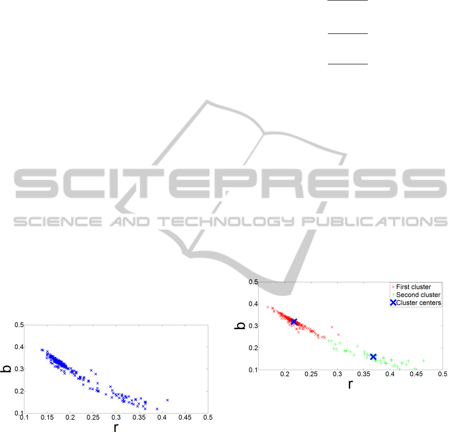
Figure 2: The rb-chromaticities of the Sony dataset (Cheng

et al., 2014b) ground-truth illuminations.

2 THE PROPOSED METHOD

2.1 Motivation

Since it is only the direction of the observed light

source e that matters, chromaticity can be used to

describe illumination. The rgb chromaticity compo-

nents of a color described by its RGB components are

calculated by scaling the RGB components so that the

equation r + g + b = 1 holds:

r =

R +G +B

, (3)

g =

R +G +B

, (4)

b =

R +G +B

. (5)

Each estimation of e can result in various values.

Fig. 2 shows the ground-truth illumination chromatic-

ities for the Sony dataset (Cheng et al., 2014b). It

can be seen that there is a certain regularity that can

also be seen for any other benchmark dataset. This

has been used in (Zhang and Batur, 2014) where the

ground-truth illumination chromaticities are clustered

by performing the k-means clustering (Vassilvitskii

and University, 2007) to obtain the cluster centers,

which are used to sparsely represent the possible illu-

mination values. For a given image the cluster center

that most appropriately approximates the image scene

illumination is chosen by using the image chromatic-

ity histogram and a machine learning algorithm. In

this way the problem of illumination estimation is sig-

niﬁcantly simpliﬁed by transforming it into classiﬁca-

tion problem.

Figure 3: The Canon1 dataset (Cheng et al., 2014b) ground-

truth illumination clustering example.

Fig. 3 shows a possible clustering of the Canon1

dataset (Cheng et al., 2014b) ground-truth illumi-

nations. Since the illumination chromaticities are

densely placed together, representing any of them

with one member of a well chosen small set of illu-

mination chromaticities results in only a small error

and consequently in a good approximation. This was

done in (Zhang and Batur, 2014), but the method de-

scribed there is a learning-based method that is not

very appropriate for devices with limited computa-

tional power.

As seen in Fig. 4, the illumination estimations

chromaticities of White-patch and Gray-world are

scattered around the ground-truth illumination chro-

maticities. Similar arrangements can be observed for

VISAPP2015-InternationalConferenceonComputerVisionTheoryandApplications

130

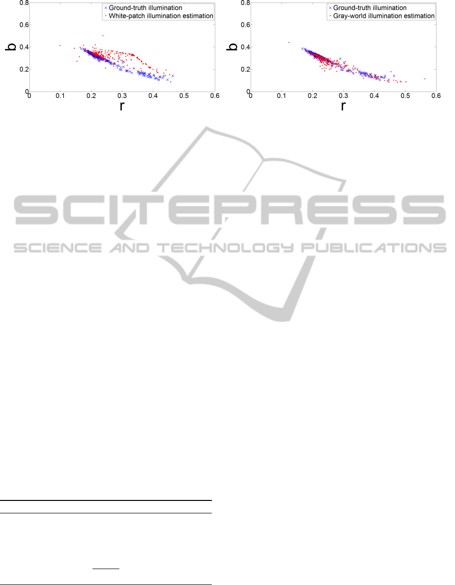
(a) (b)

Figure 4: The illumination estimation rb-chromaticities on the Canon1 dataset (Cheng et al., 2014b) for (a) White-patch and

(b) Gray-world method.

other methods as well. Such arrangements lead to the

motivation of trying to correct the methods’ illumina-

tion estimations by getting their chromaticities closer

to the region occupied by the ground-truth illumina-

tion chromaticities.

2.2 Realisation

Instead of performing classiﬁcation by extracting fea-

tures and applying a machine learning algorithm, we

propose a method that chooses the most appropriate

center by performing a voting where the voters are

some existing illumination estimation methods that

cast a vote of different strength for each of the avail-

able centers. Since both the methods’ illumination

estimations and the centers are vectors, the vote that

each of the used methods casts for each of the cen-

ters can be deﬁned as the cosine of the angle between

the center and the method’s illumination estimation.

The center with the maximum sum of the votes is the

proposed method’s illumination estimation.

Since dogs are known for their leading abilities

and the proposed method leads the voters’ illumina-

tion estimations to higher accuracy, it was named the

Color Dog (CD). The pseudocode for the application

phase of the Color Dog method is given in Algo-

rithm 1. An example of Color Dog correction with

only one voter is shown in Fig. 5.

Algorithm 1: Color Dog Application.

1: I = GetImage()

2: for all voter

∈ {voter

, ..., voter

} do

3: e

= voter

.EstimateIllumination(I)

4: end for

5: e = argmax

c∈centers



∑

i=1

c·e

||c||·||e



The voters are chosen by considering where the

illumination estimation is to be applied. on digital

cameras it might be better to use statistics-based vot-

ers since they are fast. If speed is not critical, then cor-

rection the illumination estimation of learning-based

methods might result in an even higher accuracy. If

the Color Dog uses used voters v

, v

, ..., v

, then this

the notated as CD

,...,v

In addition to any parameters of the voter meth-

ods, the center positions also need to be learned.

This is done by performing k-means algorithm on the

ground-truth illuminations of the learning set. Addi-

tionally, what also needs to be determined is the num-

ber of centers, which is a hyperparameter and each

value represents a different model. More centers re-

sult in a more accurate chromaticity space represen-

tation and a harder classiﬁcation problem, so the op-

timal number of centers has to be chosen carefully.

This is done in the model selection process (Japkow-

icz and Shah, 2011), which conducts a grid search

guided by cross-validating the proposed method for

a given number of centers. At the end the selected

model i.e. number of centers is the one that resulted

in the lowest generalization error.

3 EXPERIMENTAL RESULTS

3.1 Benchmark Datasets

Since the image formation model used in Eq. (1) is

linear and in digital cameras color constancy methods

are implemented to work on linear images (Gijsenij

et al., 2011), datasets with linear image were used to

test the accuracy of the proposed method in such en-

vironments. Until recently the only publicly available

and well-known raw-based dataset with linear im-

ages was the Shi’s and Funt’s re-processed linear ver-

sion (L. Shi, 2014) of the ColorChecker dataset (Gi-

jsenij and Gevers, 2007). However, in most publi-

cations this dataset was used without subtracting the

black level (Lynch et al., 2013), which led to wrong

ColorDog-GuidingtheGlobalIlluminationEstimationtoBetterAccuracy

131

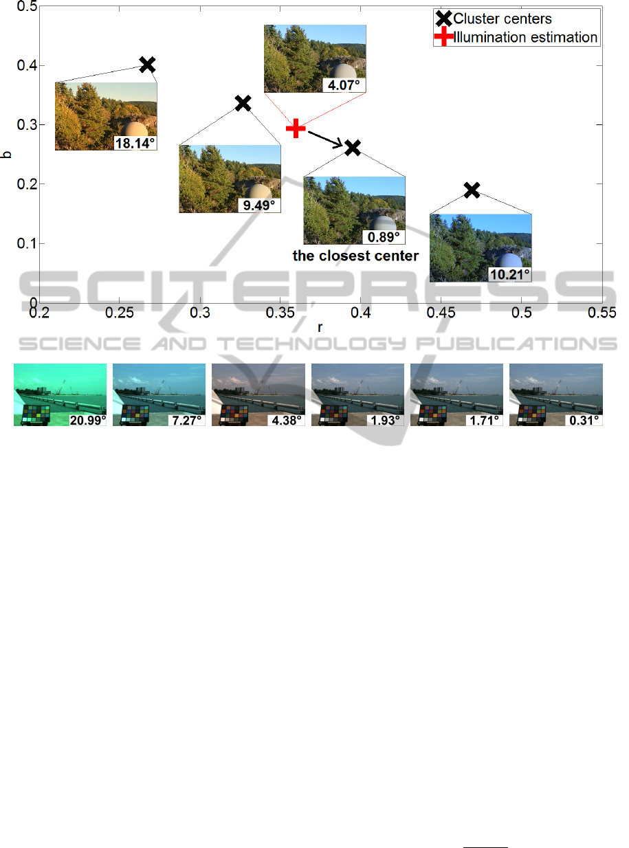
Figure 5: Example of the Color Dog method with one voter choosing the closest center.

(a) (b) (c) (d) (e) (f)

Figure 6: Example of chromatic adaptation based on the methods’ illumination estimation and respective illumination esti-

mation errors: (a) do nothing, (b) White-patch, (c) Gray-world, (d) Color Distribution, (e) Color Rabbit), and (f) proposed

method.

estimations. Since this might lead to certain com-

parison problems, the linear ColorChecker was not

used. Instead the nine new NUS datasets (Cheng

et al., 2014b) were used. Images of these datasets are

of high-quality and each dataset corresponds to a dif-

ferent camera. In addition to these datasets, the non-

linear GreyBall dataset (Ciurea and Funt, 2003) and

its approximated linear version were used because

they are the largest available benchmark datasets.

In the scene of each image is a calibration ob-

ject used to extract the ground-truth illumination of

the scene. When an illumination estimation method

is applied to the image, the calibration object is ﬁrst

masked out in order to avoid bias. After the illumi-

nation estimation is performed, the angle between the

resulting vector and the ground-truth vector is calcu-

lated and used as the error measure i.e. as angular er-

ror. The commonly used statistics descriptor used to

describe a method’s performance on a dataset is the

median of per image angular error (Hordley and Fin-

layson, 2004). The mean is less important because

the angular error distribution is in many cases non-

symmetric.

3.2 Used Voters

Because speed is a desirable feature of illumination

estimation methods, especially for real-time embed-

ded system implementations, one of the tested Color

Dog voter method sets contained two of the sim-

plest methods that have no parameters: White-patch

and Gray-world method. They are very fast, but not

very accurate and any improvement of their accuracy

is signiﬁcant. White-patch illumination estimation

looks like this:





max f





, (6)

but for better performance, clipped pixels should be

excluded from the maxima calculation (Funt and Shi,

2010). Gray-world illumination estimation is per-

formed in the following way:

f(x)dx

. (7)

VISAPP2015-InternationalConferenceonComputerVisionTheoryandApplications

132

Table 1: Angular error of selected low-level statistics-based methods, the proposed method, and selected learning-based

methods on nine NUS benchmark image databases (lower is better).

Low-level statistics-based methods Learning-based methods

Method CR CD GW WP GGW GE1 GE2 CD

GW,W P

PG EG IG ML GP NIS

Dataset Mean angular error (

◦

)

Canon1 3.09 2.93 5.16 7.99 3.16 3.45 3.47 3.13 6.13 6.07 6.37 3.58 3.21 4.18

Canon2 2.81 2.81 3.89 10.96 3.24 3.22 3.21 2.83 14.51 15.36 14.46 2.80 2.67 3.43

Fuji 2.94 3.15 4.16 10.20 3.42 3.13 3.12 3.36 8.59 7.76 6.80 3.12 2.99 4.05

Nikon1 3.06 2.90 4.38 11.64 3.26 3.37 3.47 3.19 10.14 13.00 9.67 3.22 3.15 4.10

Oly 2.65 2.76 3.44 9.78 3.08 3.02 2.84 2.57 6.52 13.20 6.21 2.92 2.86 3.22

Pan 2.89 2.96 3.82 13.41 3.12 2.99 2.99 2.84 6.00 5.78 5.28 2.93 2.85 3.70

Sam 2.94 2.91 3.90 11.97 3.22 3.09 3.18 2.92 7.74 8.06 6.80 3.11 2.94 3.66

Sony 2.88 2.93 4.59 9.91 3.20 3.35 3.36 2.83 5.27 4.40 5.32 3.24 3.06 3.45

Nikon2 3.57 3.81 4.60 12.75 4.04 3.94 3.95 3.37 11.27 12.17 11.27 3.80 3.59 4.36

Dataset Median angular error (

◦

)

Canon1 2.08 2.01 4.15 6.19 2.35 2.48 2.44 1.72 4.30 4.68 4.72 2.80 2.67 3.04

Canon2 1.86 1.89 2.88 12.44 2.28 2.07 2.29 1.85 14.83 15.92 14.72 2.32 2.03 2.46

Fuji 1.84 2.15 3.30 10.59 2.60 1.99 2.00 1.81 8.87 8.02 5.90 2.70 2.45 2.95

Nikon1 1.91 2.08 3.39 11.67 2.31 2.22 2.19 1.94 10.32 12.24 9.24 2.43 2.26 2.40

Oly 1.79 1.87 2.58 9.50 2.15 2.11 2.18 1.46 4.39 8.55 4.11 2.24 2.21 2.17

Pan 1.70 2.02 3.06 18.00 2.23 2.16 2.04 1.69 4.74 4.85 4.23 2.28 2.22 2.28

Sam 1.88 2.03 3.00 12.99 2.57 2.23 2.32 1.89 7.91 6.12 6.37 2.51 2.29 2.77

Sony 2.10 2.33 3.46 7.44 2.56 2.58 2.70 1.77 4.26 3.30 3.81 2.70 2.58 2.88

Nikon2 2.42 2.72 3.44 15.32 2.92 2.99 2.95 2.12 10.99 11.64 11.32 2.99 2.89 3.51

Dataset Trimean angular error (

◦

)

Canon1 2.56 2.22 4.46 6.98 2.50 2.74 2.70 2.08 4.81 4.87 5.13 2.97 2.79 3.30

Canon2 2.17 2.12 3.07 11.40 2.41 2.36 2.37 2.07 14.78 15.73 14.80 2.37 2.18 2.72

Fuji 2.13 2.41 3.40 10.25 2.72 2.26 2.27 2.20 8.64 7.70 6.19 2.69 2.55 3.06

Nikon1 2.23 2.19 3.59 11.53 2.49 2.52 2.58 2.14 10.25 11.75 9.35 2.59 2.49 2.77

Oly 2.01 2.05 2.73 9.54 2.35 2.26 2.20 1.72 4.79 10.88 4.63 2.34 2.28 2.42

Pan 2.12 2.31 3.15 14.98 2.45 2.25 2.26 1.87 4.98 5.09 4.49 2.44 2.37 2.67

Sam 2.18 2.22 3.15 12.45 2.66 2.32 2.41 2.05 7.70 6.56 6.40 2.63 2.44 2.94

Sony 2.26 2.42 3.81 8.78 2.68 2.76 2.80 2.03 4.45 3.45 4.13 2.82 2.74 2.95

Nikon2 2.67 3.10 3.69 13.80 3.22 3.21 3.38 2.38 11.11 12.01 11.30 3.11 2.96 3.84

The described combination of the voters CD

W P,GW

was tested on all used datasets with the goal of exam-

ining how much can the accuracy of some of the sim-

plest and least accurate methods be improved with the

computational cost almost intact. For the challenging

GreyBall dataset the combinations CD

and CD

were also tested where the voter methods described

in (Joze and Drew, 2012) and (Bani

c and Lon

cari

2015) were used to examine if the accuracy of already

successful methods can be improved even further.

3.3 Accuracy

Table 1 shows the error statistics achieved on the

NUS datasets, Table 2 on the original GreyBall

dataset, and Table 3 on its linear version. The re-

sults for other methods were taken from (Cheng et al.,

2014b) (Cheng et al., 2014a) (A. Gijsenij and van de

Weijer, 2014). Because the proposed method is a

learning one, like for other learning-based methods

the 3-fold cross-validation was used on the NUS

Table 2: Performance of different color constancy methods

on the original GreyBall dataset (lower is better).

method mean (

◦

) median (

◦

) trimean (

◦

)

do nothing 8.28 6.70 7.25

Low-level statistics-based methods

GW 7.87 6.97 7.14

WP 6.80 5.30 5.77

SoG 6.14 5.33 5.51

general GW 6.14 5.33 5.51

GE1 5.88 4.65 5.11

GE2 6.10 4.85 5.28

Learning-based methods

PG 7.07 5.81 6.12

EG 6.81 5.81 6.03

IG 6.93 5.80 6.05

NIS 5.19 3.93 4.31

EB 4.38 3.43 3.67

CC 4.22 3.17 3.46

W P,GW

5.27 3.71 4.16

4.68 3.11 3.72

4.50 2.86 3.50

ColorDog-GuidingtheGlobalIlluminationEstimationtoBetterAccuracy

133

Table 3: Performance of different color constancy methods

on the linear GreyBall dataset (lower is better).

method mean (

◦

) median (

◦

) trimean (

◦

)

do nothing 15.62 14.00 14.56

Low-level statistics-based methods

GW 13.01 10.96 11.53

WP 12.68 10.50 11.25

SoG 11.55 9.70 10.23

general GW 11.55 9.70 10.23

GE1 10.58 8.84 9.18

GE2 10.68 9.02 9.40

Learning-based methods

PG 11.79 8.88 9.97

EG 12.78 10.88 11.38

IG 11.81 8.93 10.00

HVLI 9.73 7.71 8.17

NIS 9.87 7.65 8.29

EB 7.97 6.46 6.77

CC 8.73 7.07 7.43

W P,GW

10.27 7.33 8.20

8.46 5.63 6.73

8.79 5.66 6.89

datasets. On the GreyBall dataset the 15-fold cross-

validation was used with the folds provided by the

authors. In the loop performing the cross-validation

there was another cross-validation to determine the

optimal number of centers so that the whole testing

was performed using a nested cross-validation.

For the most of the NUS datasets the proposed

W P,GW

outperforms all other methods in terms of

median angular error, which is a signiﬁcant result.

Since the median angular error is for all NUS datasets

below 3

◦

, which was experimentally shown to be

an acceptable error for human observers (Finlayson

et al., 2005) (Fredembach and Finlayson, 2008), the

results of CD

W P,GW

are in most cases satisfying.

Fig. 6 shows the results of chromatic adaptation based

on illumination estimation of several methods on the

NUS datasets. Beyond the fact that the CD

W P,GW

, it

also demonstrates how even very simple statistics of

a realistic illumination distribution can signiﬁcantly

improve the initially low accuracy of simple methods

up to the level to outperform state-of-the-art methods

in most cases.

For the GreyBall dataset and its linear version

W P,GW

outperformed all statistics-based methods

and compared very well with the learning-based ones

being less accurate than only a small number of them.

The other tested combination CD

outperformed all

other methods in terms of median angular error prov-

ing that already accurate methods can have their ac-

curacy improved even further in a simple way.

3.4 Computational Speed

Since the computation cost of voting is negligible,

the computational cost the Color Dog depends only

on the combined computational costs of its voters.

According to the tests performed in (Cheng et al.,

2014b) White-patch and Gray-world method are the

two fastest methods and even their combined compu-

tation time is low, so CD

W P,GW

is not only accurate,

but also a fast method suitable for implementation in

digital cameras with limited computational power.

4 CONCLUSIONS AND FUTURE

RESEARCH

A new global illumination estimation learning-based

methods has been proposed. It uses other methods’ il-

lumination estimations to vote for the most appropri-

ate illumination from a predeﬁned set with almost no

additional computational cost. The method demon-

strates how even some of the least accurate meth-

ods can be improved up to the level of outperform-

ing most of the other methods while at the same time

keeping their advantages. It also demonstrates that

the accuracy of already very accurate methods can

be improved even further. In future some more so-

phisticated and accurate voting methods should be re-

searched.

ACKNOWLEDGEMENTS

This research has been partially supported by the Eu-

ropean Union from the European Regional Develop-

ment Fund by the project IPA2007/HR/16IPO/001-

040514 ”VISTA - Computer Vision Innovations for

Safe Trafﬁc.”

REFERENCES

A. Gijsenij, T. G. and van de Weijer, J. (2014). Color Con-

stancy — Research Website on Illuminant Estimation.

Bani

c, N. and Lon

cari

c, S. (2013). Using the Random

Sprays Retinex Algorithm for Global Illumination Es-

timation. In Proceedings of The Second Croatian

Computer Vision Workshop (CCVW 2013), pages 3–7.

University of Zagreb Faculty of Electrical Engineer-

ing and Computing.

Bani

c, N. and Lon

cari

c, S. (2014a). Color Rabbit: Guid-

ing the Distance of Local Maximums in Illumina-

tion Estimation. In Digital Signal Processing (DSP),

2014 19th International Conference on, pages 345–

350. IEEE.

VISAPP2015-InternationalConferenceonComputerVisionTheoryandApplications

134

Bani

c, N. and Lon

cari

c, S. (2014b). Improving the White

patch method by subsampling. In Image Processing

(ICIP), 2014 21st IEEE International Conference on,

pages 605–609. IEEE.

Bani

c, N. and Lon

cari

c, S. (2015). Color Cat: Remember-

ing Colors for Illumination Estimation. Signal Pro-

cessing Letters, IEEE, 22(6):651–655.

Buchsbaum, G. (1980). A spatial processor model for object

colour perception. Journal of The Franklin Institute,

310(1):1–26.

Cardei, V. C., Funt, B., and Barnard, K. (2002). Estimating

the scene illumination chromaticity by using a neural

network. Journal of the Optical Society of America A,

19(12):2374–2386.

Chakrabarti, A., Hirakawa, K., and Zickler, T. (2012). Color

constancy with spatio-spectral statistics. Pattern Anal-

ysis and Machine Intelligence, IEEE Transactions on,

34(8):1509–1519.

Cheng, D., Prasad, D., and Brown, M. S. (2014a). On Illu-

minant Detection.

Cheng, D., Prasad, D. K., and Brown, M. S. (2014b). Il-

luminant estimation for color constancy: why spatial-

domain methods work and the role of the color distri-

bution. Journal of the Optical Society of America A,

31(5):1049–1058.

Ciurea, F. and Funt, B. (2003). A large image database

for color constancy research. In Color and Imaging

Conference, volume 2003, pages 160–164. Society for

Imaging Science and Technology.

Deng, Z., Gijsenij, A., and Zhang, J. (2011). Source camera

identiﬁcation using Auto-White Balance approxima-

tion. In Computer Vision (ICCV), 2011 IEEE Interna-

tional Conference on, pages 57–64. IEEE.

Ebner, M. (2007). Color Constancy. The Wiley-IS&T Se-

ries in Imaging Science and Technology. Wiley.

Finlayson, G. D., Hordley, S. D., and Morovic, P. (2005).

Colour constancy using the chromagenic constraint.

In Computer Vision and Pattern Recognition, 2005.

CVPR 2005. IEEE Computer Society Conference on,

volume 1, pages 1079–1086. IEEE.

Finlayson, G. D., Hordley, S. D., and Tastl, I. (2006). Gamut

constrained illuminant estimation. International Jour-

nal of Computer Vision, 67(1):93–109.

Finlayson, G. D. and Trezzi, E. (2004). Shades of gray and

colour constancy. In Color and Imaging Conference,

volume 2004, pages 37–41. Society for Imaging Sci-

ence and Technology.

Fredembach, C. and Finlayson, G. (2008). Bright chroma-

genic algorithm for illuminant estimation. Journal of

Imaging Science and Technology, 52(4):40906–1.

Funt, B. and Shi, L. (2010). The rehabilitation of MaxRGB.

In Color and Imaging Conference, volume 2010,

pages 256–259. Society for Imaging Science and

Technology.

Gehler, P. V., Rother, C., Blake, A., Minka, T., and Sharp, T.

(2008). Bayesian color constancy revisited. In Com-

puter Vision and Pattern Recognition, 2008. CVPR

2008. IEEE Conference on, pages 1–8. IEEE.

Gijsenij, A. and Gevers, T. (2007). Color Constancy us-

ing Natural Image Statistics. In Computer Vision and

Pattern Recognition, 2008. CVPR 2008. IEEE Confer-

ence on, pages 1–8.

Gijsenij, A., Gevers, T., and Van De Weijer, J. (2011).

Computational color constancy: Survey and exper-

iments. Image Processing, IEEE Transactions on,

20(9):2475–2489.

Gijsenij, A., Gevers, T., and Van De Weijer, J. (2012). Im-

proving color constancy by photometric edge weight-

ing. Pattern Analysis and Machine Intelligence, IEEE

Transactions on, 34(5):918–929.

Hordley, S. D. and Finlayson, G. D. (2004). Re-evaluating

colour constancy algorithms. In Pattern Recognition,

2004. ICPR 2004. Proceedings of the 17th Interna-

tional Conference on, volume 1, pages 76–79. IEEE.

Japkowicz, N. and Shah, M. (2011). Evaluating Learning

Algorithms. Cambridge University Press.

Joze, H. R. V. and Drew, M. S. (2012). Exemplar-Based

Colour Constancy. In British Machine Vision Confer-

ence, pages 1–12.

Joze, H. R. V., Drew, M. S., Finlayson, G. D., and Rey, P.

A. T. (2012). The Role of Bright Pixels in Illumina-

tion Estimation. In Color and Imaging Conference,

volume 2012, pages 41–46. Society for Imaging Sci-

ence and Technology.

L. Shi, B. F. (2014). Re-processed Version of the Gehler

Color Constancy Dataset of 568 Images.

Land, E. H. (1977). The retinex theory of color vision. Sci-

entiﬁc America.

Lynch, S. E., Drew, M. S., and Finlayson, k. G. D. (2013).

Colour Constancy from Both Sides of the Shadow

Edge. In Color and Photometry in Computer Vision

Workshop at the International Conference on Com-

puter Vision. IEEE.

Van De Weijer, J., Gevers, T., and Gijsenij, A. (2007a).

Edge-based color constancy. Image Processing, IEEE

Transactions on, 16(9):2207–2214.

Van De Weijer, J., Schmid, C., and Verbeek, J. (2007b). Us-

ing high-level visual information for color constancy.

In Computer Vision, 2007. ICCV 2007. IEEE 11th In-

ternational Conference on, pages 1–8. IEEE.

Vassilvitskii, S. and University, S. (2007). K-means: Algo-

rithms, Analyses, Experiments. Stanford University.

Zhang, B. and Batur, A. (2014). Illumination Estima-

tion Using Natural Scene Statistics. US Patent App.

14/188,670.

ColorDog-GuidingtheGlobalIlluminationEstimationtoBetterAccuracy

135