Fast Adaptive Frame Preprocessing for 3D Reconstruction
Fabio Bellavia, Marco Fanfani and Carlo Colombo
Computational Vision Group, University of Florence, Florence, Italy
Keywords:
Adaptive Frame Selection, Blur Detection, SLAM, Structure-from-Motion.
Abstract:
This paper presents a new online preprocessing strategy to detect and discard ongoing bad frames in video
sequences. These include frames where an accurate localization between corresponding points is difficult,
such as for blurred frames, or which do not provide relevant information with respect to the previous frames
in terms of texture, image contrast and non-flat areas. Unlike keyframe selectors and deblurring methods,
the proposed approach is a fast preprocessing working on a simple gradient statistic, that does not require
to compute complex time-consuming image processing, such as the computation of image feature keypoints,
previous poses and 3D structure, or to know a priori the input sequence. The presented method provides a
fast and useful frame pre-analysis which can be used to improve further image analysis tasks, including also
the keyframe selection or the blur detection, or to directly filter the video sequence as shown in the paper,
improving the final 3D reconstruction by discarding noisy frames and decreasing the final computation time
by removing some redundant frames. This scheme is adaptive, fast and works at runtime by exploiting the
image gradient statistic of the last few frames of the video sequence. Experimental results show that the
proposed frame selection strategy is robust and improves the final 3D reconstruction both in terms of number
of obtained 3D points and reprojection error, also reducing the computational time.
1 INTRODUCTION
Multi-view 3D reconstruction (Szeliski, 2010) is a re-
search field in computer vision, which has received
much attention in the last few years due to its range of
application, with impressive results (Gherardi et al.,
2010; Snavely et al., 2008). The selection of “good”
input sequences, both in terms of image quality and
frame order, is a crucial step in 3D reconstruction al-
gorithms. While close frames improve the tracking
of the corresponding points between the frames, they
also yield to non-efficient and almost redundant com-
putations and jittering effects which can degrade the
final 3D reconstruction.
According to the constraints imposed, multi-view
3D reconstruction algorithms can be divided in off-
line Structure-from-Motion (SfM) approaches (Gher-
ardi et al., 2010; Snavely et al., 2008) and real-
time sequential Simulaneous Localization and Map-
ping (SLAM) approaches (Klein and Murray, 2007;
Fanfani et al., 2013). In both approaches, different
strategies to improve the efficiency and the quality of
the reconstructed output have been investigated, by
using keyframes (Klein and Murray, 2007; Seo et al.,
2008) in the case of SLAM, or clustering (Gherardi
et al., 2010) and graph-based approaches (Snavely
et al., 2008) for SfM.
In the presence of motion blur due to fast cam-
era motion or shake, the uncertainty in the position of
corresponding points amplifies the 3D point estima-
tion error, which in some cases can lead to a camera
tracking loss and the failure of the system. Differ-
ent methods have been presented to improve the cam-
era re-localization and recovery system and to allow
a robust tracking of blurry features. These include
the use of edgelets (Klein and Murray, 2008) and
the estimation of the blur kernel to deblur the current
frame (Lee et al., 2011), incorporating camera trajec-
tory clues with blind deconvolution techniques (Joshi
et al., 2008), or to blur the previous frame in order to
obtain a consistent tracking (Mei and Reid, 2008).
Different metrics have been also investigated in
order to estimate the amount of blur in images, based
on the color saturation, local autocorrelation and gra-
dient distribution (Liu et al., 2008), or spectral and
wavelet analysis (Tong et al., 2004). In general, it
turns out that robust measures can be derived from
the gradient magnitude distribution (Liu et al., 2008),
which also can give clues about the relevant structure
of the image, in term of discriminant features, image
contrast, border and non-flat and textured areas, thus
providing robust correspondences.
260
Bellavia F., Fanfani M. and Colombo C..
Fast Adaptive Frame Preprocessing for 3D Reconstruction.
DOI: 10.5220/0005272702600267
In Proceedings of the 10th International Conference on Computer Vision Theory and Applications (VISAPP-2015), pages 260-267
ISBN: 978-989-758-091-8
Copyright
c
 2015 SCITEPRESS (Science and Technology Publications, Lda.)

This paper presents the Double Window Adaptive
Frame Selection (DWAFS) algorithm for video se-
quences based on the gradient magnitude distribution.
In particular, as shown in Sect. 2, the percentile statis-
tic computed on each frame is used to develop an
adaptive decision strategy based on a dangling sam-
ple window according to the time series of the ongo-
ing percentile values and the last best ones.
Unlike keyframe selectors and deblurring meth-
ods, DWAFS is a fast preprocessing method that does
not require to compute complex time-consuming im-
age processing, such as the computation of image fea-
ture keypoints, previous poses and 3D structure, or to
know a priori the input sequence. Nevertheless, it pro-
vides a useful and fast frame pre-analysis which can
be used to improve further image analysis tasks, in-
cluding also the keyframe selection or the blur detec-
tion, or to directly filter the video sequence as shown
in Sect. 3, improving the final 3D reconstruction by
discarding noisy frames and decreasing the final com-
putation time by removing some redundant frames.
DWAFS tries to select high-detailed and unblurred
frames, butalso to adapt to the current frame sequence
after a transition time as in the case of a switch from
highly structured and contrasted image to more flat
ones, or in the case of long-lasting camera shakes.
2 METHOD DESCRIPTION
The DWAFS method uses the p
m
percentile of the gra-
dient magnitude k ∇I
t
k of each image frame I
t
of the
video sequence V = {I
t
|t = 1,2,.. . ,n} as statistic,
m ∈ [0,100]. The spatial gradient ∇I
t
, whose direc-
tional derivatives are computed by convolution of the
image I
t
with the kernel masks [−1 1] and [−1 1]
T
respectively, gives a fast robust estimation of the im-
age blur (Liu et al., 2008), but also provides clues
about the relevant structure of the image, such as bor-
ders and salient features (Szeliski, 2010). Figure 1
shows the Matlab code of DWAFS while an example
of the DWAFS steps for two successive frames I
t
,I
t+1
is given in Fig. 2.
At each time step t > w, the DWAFS algorithms
considers two different samples of size w in order to
make a decision on the frame I
t
. Note that for t ≤ w
no output is given (line 12). The current sample C
t
(line 15) contains the gradient percentile values of the
last w frames
C
t
= {p
t−w+i
|i = 1, 2, ... ,w} (1)
i.e. a running window of size w is considered, where
p
t
= p
m
(k ∇I
t
k). The best sample B
t
(lines 13, 22)
DWAFS Matlab code
1 function S=dwafs(p,w)
2 % input:
3 % - p (1xn double array) gradient percentiles
4 % - w (integer) window size
5 % output:
6 % - S (1xn boolean array) good frame set
7
8
S=zeros(size(p));
9 B=[];
10 d=w;
11 for t=1:length(p);
12 if t<=w
13 B=[B p(t)];
14 else
15 C=p(t-w+1:t);
16 A=sort([C B]);
17 F=A(ceil(d)+1:ceil(d)+w);
18 m=mean(F);
19 s=std(F);
20 if p(t)>m-2*s
21 S(t)=1;
22 B=[B(2:end) p(t)];
23 d=min(w,d+1);
24 else
25 d=max(0,d-0.5);
26 end;
27 end;
28 end;
Figure 1: DWAFS Matlab code.
contains the gradient percentile values of the previ-
ously w selected frames
B
t
= {p
k
z−w+i
|i = 1, 2, ... ,w}, (2)
where S
t
= {I
k
1
,I
k
2
,. .. ,I
k
z
} is the time-ordered set of
the previous good selected frames, with k
1
< k
2
<
·· · < k
z
≤ z < t and k
i
= i for 1 ≤ i ≤ w.
The sorted list A
t
(line 16), obtained by merging
both the elements of B
t
and C
t
ordered according to
8 93
5
4 4
6
5
2 3
3
4
5
5
6 9
5
3
44
9
8 6 20
1
4
5
3
98
4
6
1
0 2
Figure 2: An example of the DWAFS frame processing for
two successive frames I
t
,I
t+1
with a windows of size w = 4.
The sample windows C
t
, B
t
and F
t
(see text) are shown in
red, green and blue respectively, the window shift of F
t
is
represented by the dashed blue window. In the case shown,
frame I
t
is selected while frame I
t+1
is dropped (best viewed
in color).
FastAdaptiveFramePreprocessingfor3DReconstruction
261

0 50 100 150 200 250 300 350 400 450 500
0.16
0.18
0.2
0.22
0.24
0.26
0.28
0.3
0.32
0.34
a
b
c
d
e
f
frame index t
k ∇I
t
k
a
b
c
d
e
f
p
m
t
DWAFS
F
t
C
t
B
t
A
t
B
⋆
t
G
t
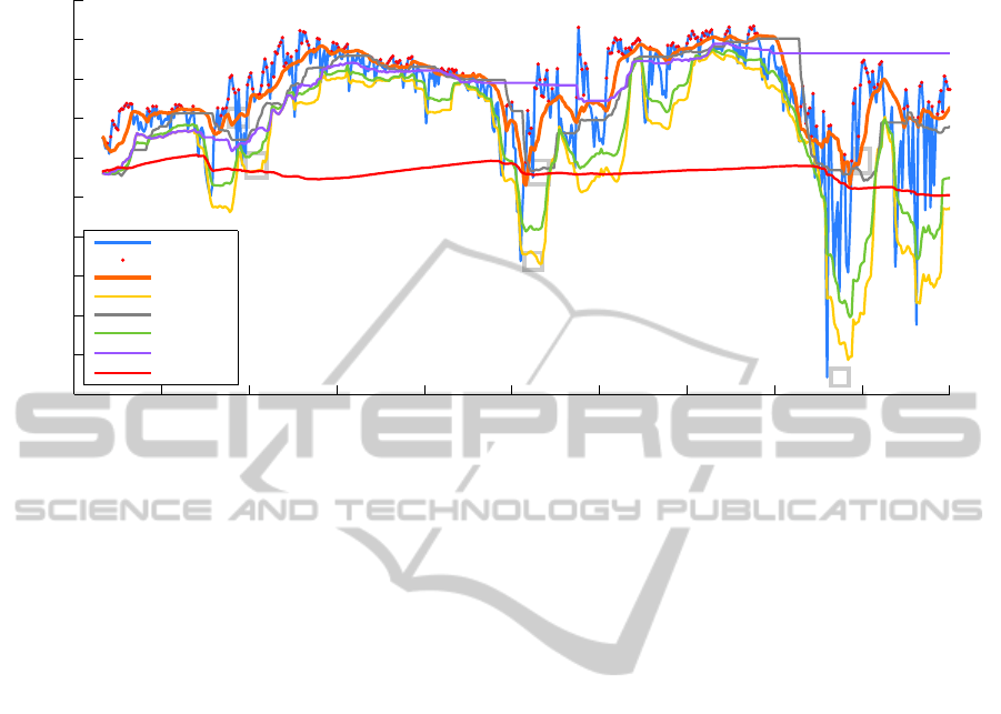
Figure 3: Plot of the gradient percentiles k ∇I
t
k with respect to the frame index t for the Monk video sequence with m = 0.95
and w = 15 as the video frame rate (best viewed in color). DWAFS selected frames and thresholds of the kind µ(W
t
)− 2σ(W
t
)
for different sample windows W
t
are reported, too (best viewed in color).
the percentile value
A
t
= B
t
⊕C
t
=
= {p
a
i
| p
a
i
≤ p
a
i+1
∧ i = 1,2,. ..,2w}
(3)
is used to get the final list of samples F
t
(line 17)
F
t
= {p
a
⌈d
t
⌉+i
|i = 1,2,.. .,w} (4)
where d
t
is a dangling factor used to adapt the final
sample list F
t
as the video sequence varies, recur-
sively defined (lines 10, 23, 25) as
d
t
=



w if t = w+ 1
min(w, d
t−1
+ 1) if I
t−1
∈ S
t
max(0,d
t−1
− 1/2) if I
t−1
/∈ S
t
(5)
i.e. the dangling window that defines F
t
on A
t
is
shifted towards high sample values if the previous
frame I
t−1
was retained as good, or to lower values
otherwise. Note that in order to support stationary and
more conservative conditions, the extent of the shift is
not symmetric.
Specifically, from the rightmost window position
2w frame drops are needed to move towards the left-
most window position, while only w successive good
frame selections are needed for the opposite direction.
Finally, the frame I
t
is kept as good if (line 20)
p
t
> µ
t
− 2σ
t
(6)
where µ
t
,σ
t
are respectively the mean and standard
deviation of F
t
(lines 18–19). The final sample list F
t
moves smoothly between the sampling sets C
t
and B
t
in order to adapt to changes in the video sequences.
Furthermore, any frame which is both considered
good (i.e. contained in B
t
) and still contained in the
current window C
t
is weighted twice in F
t
, since it
appears duplicated in A
t
.
Figure 3 shows a DWAFS run over a video se-
quence. Thresholds of the kind µ(W
t
) − 2σ(W
t
) for
different sample windows W
t
are also shown, corre-
sponding to different possible frame selection strate-
gies. Beside the sample windows C
t
, B
t
, A
t
and F
t
,
the thresholds in the case of the best window B
⋆
t
, i.e.
B
t
is used in the place of F
t
in DWAFS, and of the on-
going window G
t
= {p
i
|i = 0,1,. ..,i} are presented.
Image details for labeled frames of the sequences are
also shown in Fig. 4. Note that while the discarded
frame (b) looks similar to the accepted frames (d) and
(f), also in terms of gradient percentiles, the running
video sequence context is different. Indeed, frame
(b) comes slightly after a better frame subsequence
whose frame (a) is a representative, while frame (d)
and frame (f) come after very blurry subsequences
represented respectively by frames (c) and (e).
The B
⋆
t
window sample in Fig. 3 (purple dashed
line) cannot take into account rapid scene change to-
wards low gradient, while a strictly local sample such
as for C
t
(yellow dashed line), is too permissive, as
well as the full-length sample of G
t
(red dashed line),
which cannot be so responsive to adapt to the scene.
The B
t
sample window (gray dashed line) is slightly
more selective than C
t
but it cannot handle a rapid
VISAPP2015-InternationalConferenceonComputerVisionTheoryandApplications
262

(a) (b)
(c) (d)
(e) (f)
Figure 4: Image details for some frames of video sequence
of Fig. 3, selected by DWAFS ((a),(d),(f)) and dropped
((b),(c),(e)) (best viewed in color).
decrease of gradient (see values around t = 425) and
an the A
t
sample (green dashed line) is an average
between C
t
and B
t
. DWAFS final sample F
t
(orange
dashed line) responds better than others, also due to
the double weighting of the samples both contained
in C
t
and B
t
.
It is worth nothing that using the average values
of the window samples instead of a combination of
the mean and the standard deviation (not shown in the
plot) would not be a good idea. Indeed, since the av-
erage value of a line slope is in the middle, it would
be a value too low and permissive when the curve in-
creases and a value too high and restrictive when the
curve decreases.
3 EVALUATION
3.1 Experimental Setup
Four video sequences lasting about 1 minute each,
with a resolution of 640× 480 pixels exploring two
different indoor scene were used (see Fig. 5) to
demonstrate the effective benefits of DWAFS. The
first three sequences, named Desktop0, Desktop1 and
Desktop2 (see Fig. 5(a)), explore the same desktop
environment as the camera undergoes to different mo-
tion speeds, so that motion blur effects and shakes de-
crease from Desktop0 to Desktop2, and are recorded
at 30 fps. The last Monk sequence (see Fig. 5(b)),
taken at 15 fps, shows an object continuously ob-
served from different viewpoints.
(a)
(b)
Figure 5: Snapshots of the environment of Desktop0, Desk-
top1 and Desktop2 example1 and of the Monk sequence ex-
ample2.
Two different kinds of reconstruction tests were
done. In one case, the 3D reconstruction results
obtained using the whole sequence V = {I
t
|t =
1,2,.. .,n}, the set of frames selected by DWAFS
S = S
n+1
(see Sect. 2) and its complement C = V \ S
were compared. In the other case, the uniform deci-
mated video sequence V
r
V
r
= {I
t
|t = 1 + ir ∧ i = 0,1,.. .,⌊n/(r− 1)⌋} (7)
generated from V by a stride of r frames, is compared
with the corresponding DWAFS decimated frame
subset S
r
⊆ S of DWAFS frames temporally close to
FastAdaptiveFramePreprocessingfor3DReconstruction
263

V
r
, so that a frame I
t
belong to S
r
only if the distance
|t − k| for a frame I
k
∈ V
r
is the minimal among all
the frames in S.
In both tests w was heuristically set to the video
frame rate, since it implies a reasonable camera shake
of about 1s, while in the decimated test r = ⌈w/2⌉.
For this setup it was experimentally verified that |S| ≃
|V|/2 while the maximum distance equals roughly the
video frame rate. This also implies a four times faster
computation, as 3D reconstruction algorithms have a
time complexity of at least O(n
2
).
The 3D reconstruction was achieved by using the
state-of-the-art freely available SfM pipeline Visu-
alSFM (Wu, 2013) where matches between keypoints
are computed on a window of h successive frames,
where h = 7 for the Monk sequence and h = 13 for the
other video sequences. Note that the windows size is
intended in terms of successive frames given as input
to VisualSFM. In the case of the full sequence V, the
window size is doubled in order to preserve the spatial
consistency between the frame matches.
No further methods are included in the evalua-
tion, since no other similar methods exist to the best
of our knowledge, and a comparison with keyframe
selection strategies (Seo et al., 2008) or deblurring
methods (Lee et al., 2011) would be unfair as they
differ in purposes and use additional information. In
particular, DWAFS aims at providing a fast data pre-
processing to be used for other tasks, working on a
simple gradient statistic, that does not require com-
plex time-consuming image processing, as the com-
putation of image feature keypoints, previous poses
and 3D structure as most of keyframe selectors and
deblurring methods, which represent possible final
tasks which can benefit of DWARF.
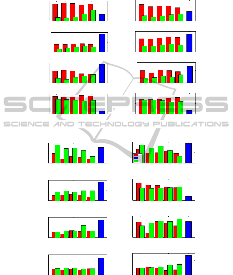
3.2 Results
Results in the case of the full and decimated se-
quences are reported respectively in Figs. 6 and 7.
In particular, the histograms of the total number of
3D point of the reconstructed model are reported, as
well as the corresponding mean reprojection error and
the track length associated, together with the aver-
age number of feature points found on each frame.
Note that for the full sequence V, the average track
length bar is halved to get the same frame spatial track
length, since V frames are about twice those of S and
C.
Reasonably, it can be stated that the product of the
average track length times the number of 3D points
must be roughly equals to product of the mean num-
ber of features per images times the total number of
image frames. So, in order to provide a more accu-
rate, defined and dense 3D reconstruction, not only
a higher number of 3D points must be found, but
also more features on the images or longer tracks.
Both cases improve the reconstruction accuracy and
decrease the estimation errors, by providing a denser
3D point cloud in the former case or a more robust
and stable reconstruction in the latter case.
Referring to Fig. 6, the DWAFS strategy notably
improves the reconstruction in the case of the Monk
and Desktop2 sequences. The relatively small de-
crease of the average track length can be attributed
to a major number of features found on images. More
robust and stable point are retained first so that im-
provements can be only done by adding points last-
ing less on the sequence with clearly shorter tracks,
decreasing the average track length. Nevertheless, re-
projection error still remains lower.
In the case of the Desktop0 and Desktop1, al-
though with respect to the full sequence V less 3D
points are found, an higher number of features with
longer track lengths are found in the image, which
together with a lower reprojection error means that
the V models contain fragmented and unstable tracks.
This implies that multiple tracks are associated to the
same 3D point which appears duplicated, that implies
a misleading untrue denser model.
Concerning the comparison between the DWAFS
sequence S and its complement C, there is noticeable
difference between them for fast camera movements
and shakes with noticeable blur (Monk, Desktop0 and
Desktop1 videos). Also for slow camera movements
(Desktop2 sequence), although reduced, better results
are obtained for S. Note that the reprojection error for
C is lower then that of the full sequences V as this got
a higher number of points per image. Nevertheless,
the reprojection error ofC is higher than that of S even
if there is an higher number of points per image for the
DWAFS sequence S.
Finally, from Fig. 7 it can be observed that better
3D reconstructions are obtained in the case of deci-
mated sequences. The difference lowers as the video
contains slow camera movements, in that case results
are quite similar. Note that in the decimated case
denser 3D models are found with respect to the full
image sequence, since less dense sequences are used
with the same frame windows h (see Sect. 3.1) to get
the feature matches, that implies higher effective spa-
tial window.
Moreover, by inspecting all histograms, the per-
centile parameter m seems to be quite stable, provid-
ing a peak for m = 95.
VISAPP2015-InternationalConferenceonComputerVisionTheoryandApplications
264

Total number of 3D pts Avg pts per image
Monk
80 85 90 95 98 n.d.
700
2700
4600
percentile m
3D pts
80 85 90 95 98 n.d.
100
400
700
percentile m
img pts
Desktop0
80 85 90 95 98 n.d.
10100
19300
28500
percentile m
3D pts
80 85 90 95 98 n.d.
300
500
700
percentile m
img pts
Desktop1
80 85 90 95 98 n.d.
5500
7100
8700
percentile m
3D pts
80 85 90 95 98 n.d.
500
800
1000
percentile m
img pts
Desktop2
80 85 90 95 98 n.d.
2200
5900
9600
percentile m
3D pts
80 85 90 95 98 n.d.
300
600
900
percentile m
img pts
Avg reproj. error per 3D pt Avg track length
Monk
80 85 90 95 98 n.d.
0.26
0.31
0.37
percentile m
error (px)
80 85 90 95 98 n.d.
20
40
60
percentile m
track len
S
V
C
Desktop0
80 85 90 95 98 n.d.
0.37
0.44
0.51
percentile m
error (px)
80 85 90 95 98 n.d.
9
12
16
percentile m
track len
Desktop1
80 85 90 95 98 n.d.
0.37
0.46
0.56
percentile m
error (px)
80 85 90 95 98 n.d.
25
30
35
percentile m
track len
Desktop2
80 85 90 95 98 n.d.
0.30
0.60
0.80
percentile m
error (px)
80 85 90 95 98 n.d.
40
60
70
percentile m
track len
Figure 6: Evaluation of the 3D reconstruction results on the full test video sequences. The histograms of the total number of
3D points found, the average number of points for each image frame, the mean reprojection error for each 3D point and the
average track length are reported for the full sequences V, DWAFS frames S and the complementary sets C (best viewed in
color).
FastAdaptiveFramePreprocessingfor3DReconstruction
265

Total number of 3D pts Avg pts per image
Monk
80 85 90 95 98 n.d.
4500
5200
5900
percentile m
3D pts
80 85 90 95 98 n.d.
860
960
1050
percentile m
img pts
Desktop0
80 85 90 95 98 n.d.
6100
6900
7600
percentile m
3D pts
80 85 90 95 98 n.d.
380
430
480
percentile m
img pts
Desktop1
80 85 90 95 98 n.d.
6400
6600
6800
percentile m
3D pts
80 85 90 95 98 n.d.
970
990
1010
percentile m
img pts
Desktop2
80 85 90 95 98 n.d.
9800
10000
10300
percentile m
3D pts
80 85 90 95 98 n.d.
1111
1118
1125
percentile m
img pts
Avg reproj. error per 3D pt Avg track length
Monk
80 85 90 95 98 n.d.
0.28
0.30
0.31
percentile m
error (px)
80 85 90 95 98 n.d.
12
14
16
percentile m
track len
S
r
V
r
Desktop0
80 85 90 95 98 n.d.
0.27
0.29
0.31
percentile m
error (px)
80 85 90 95 98 n.d.
3.4
3.6
3.8
percentile m
track len
Desktop1
80 85 90 95 98 n.d.
0.33
0.35
0.37
percentile m
error (px)
80 85 90 95 98 n.d.
6.07
6.14
6.22
percentile m
track len
Desktop2
80 85 90 95 98 n.d.
0.37
0.38
0.40
percentile m
error (px)
80 85 90 95 98 n.d.
8.22
8.3
8.39
percentile m
track len
Figure 7: Evaluation of the 3D reconstruction results on the decimated test video sequences. The histograms of the total
number of 3D points found, the average number of points for each image frame, the mean reprojection error for 3D point and
the average track length are reported for the uniform decimated video sequences V
r
and DWAFS decimated frames S
r
(best
viewed in color).
VISAPP2015-InternationalConferenceonComputerVisionTheoryandApplications
266

4 CONCLUSION AND FUTURE
WORK
This paper presented the DWAFS frame selection
strategy, based on the gradient, to improve the 3D re-
construction of SfM and SLAM approaches both in
terms of accuracy, point density and computational
time from video sequences. This is done by drop-
ping blurred frames or those which do not provide
further information with respect to the current video
sequence history. DWAFS provides a useful and fast
frame pre-analysis which can be used to improve fur-
ther image analysis tasks and, unlike keyframe selec-
tors and deblurring methods, it does not require to
compute complex time-consuming image processing,
such as the computation of image feature keypoints,
previous poses and 3D structure, or to known a pri-
ori the input sequence. Experimental evaluation show
that it is robust, stable and effective. Future work
will include more experimental evaluation to assess
the validity of the DWAFS approach when embed-
ded in keyframe selection methods, so that bad frames
discarded by DWAFS cannot be given as input to the
keyframe selector.
ACKNOWLEDGEMENT
This work has been carried out during the ARROWS
project, supported by the European Commission un-
der the Environment Theme of the “7th Framework
Programme for Research and Technological Develop-
ment”.
REFERENCES
Fanfani, M., Bellavia, F., Pazzaglia, F., and Colombo, C.
(2013). SAMSLAM: Simulated annealing monocu-
lar SLAM. In Proc. of 15th International Conference
on Computer Analysis of Images and Patterns, pages
515–522.
Gherardi, R., Farenzena, M., and Fusiello, A. (2010). Im-
proving the efficiency of hierarchical Structure-and-
Motion. In Proc. of Computer Vision and Pattern
Recognition, pages 1594–1600.
Joshi, N., Szeliski, R., and Kriegman, D. J. (2008). PSF es-
timation using sharp edge prediction. In Proc. of IEEE
Conference on Computer Vision and Pattern Recogni-
tion.
Klein, G. and Murray, D. (2007). Parallel tracking and map-
ping for small AR workspaces. In Proc. of IEEE/ACM
International Symposium on Mixed and Augmented
Reality, pages 225–234.
Klein, G. and Murray, D. (2008). Improving the agility of
keyframe-based SLAM. In Proc. of 10th European
Conference on Computer Vision, pages 802–815.
Lee, H. S., Kwon, J., and Lee, K. M. (2011). Simultane-
ous localization, mapping and deblurring. In Proc. of
IEEE International Conference on Computer Vision,
pages 1203–1210.
Liu, R., Li, Z., and Jia, J. (2008). Image partial blur detec-
tion and classification. In Proc. of Computer Vision
and Pattern Recognition.
Mei, C. and Reid, I. (2008). Modeling and generating com-
plex motion blur for real-time tracking. In Proc. of
Computer Vision and Pattern Recognition.
Seo, Y., Kim, S., Doo, K., and Choi, J. (2008). Optimal
keyframe selection algorithm for three-dimensional
reconstruction in uncalibrated multiple images. Op-
tical Engineering, 47(5):053201–053201–12.
Snavely, N., Seitz, S. M., and Szeliski, R. (2008). Skeletal
graphs for efficient structure from motion. In Proc. of
Computer Vision and Pattern Recognition, pages 1–8.
Szeliski, R. (2010). Computer Vision: Algorithms and Ap-
plications. Springer-Verlag New York, Inc., 1st edi-
tion.
Tong, H., Li, M., Zhang, H., and Zhang, C. (2004). Blur
detection for digital images using wavelet transform.
In Proc. of IEEE International Conference on Multi-
media & Expo, pages 17–20.
Wu, C. (2013). Towards linear-time incremental structure
from motion. In Proc. of Joint 3DIM/3DPVT Confer-
ence.
http://ccwu.me/vsfm/ .
FastAdaptiveFramePreprocessingfor3DReconstruction
267