
Best Path Selection in a Multi-Relay Node System under the
Concept of Cognitive Radio
Zaid A. Shafeeq
1
, Ghazi M. AL Sukkar
2
and Ahmad ALAmayreh
1
1
Department of Electronics and Communication Engineering, Al-Ahliyya Amman University, Amman, Jordan
2
Department of Electrical Engineering, The University of Jordan, Amman, Jordan
Keywords: Relay Technology, Cognitive Radio, Path Selection.
Abstract: The main purpose in this work is to enhance relay technique in underlay cognitive radio scheme through
estimating the best path between the secondary source and the secondary destination under the power
interference constraint of the primary user. A protocol is proposed based on the cooperation process
between the secondary relay nodes in the system in order to establish the best path at low complexity
without exceeding the interference threshold of the primary user. Performance analyses, through simulation,
of the suggested protocol shows great enhancement in network outage probability when compared with
direct path model and one relay node based-model.
1 INTRODUCTION
In the last years, wireless communications systems
have experienced sharp growth, as there are around
seven billion users around the world. Providing the
service of mobile access in wireless communications
systems to such a large number of users requires a
solution to the wide spectrum issues from both
scientific and economic aspects. New technologies
in wireless communications systems must be
developed in order to enhance the quality of service
(QoS), the throughput and the reliability of
communication networks (Goldsmith, 2005).
One of the basic challenges that face the
developers is supplying high throughput at the cell
edge (Goldsmith, 2005), (Mikio, 2010). Relay
technology provides solutions that have been applied
to improve the coverage at the cell edge (Klaus,
2010).
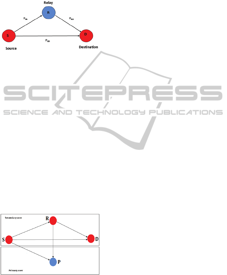
The main idea behind the relay technology is a
cooperation process that depends on the nodes
located in the distance between the source and the
destination. These relay nodes receive the signal
from the source and they transmit it to the receiver
as shown in figure1, where
,
and
represent the paths between the source and the relay,
the relay and the destination and the source and the
destination respectively.
On the other hand, to overcome the shortage on
the frequency spectrum and to enhance its
utilization, cognitive radio technology has been
developed in the past few years. Cognitive radio is
simply one of the forms of wireless communications
where in one of its three well-known schemes, the
basic scheme (called interweave), the secondary user
(the unlicensed user to use the spectrum) can
intelligently detect and distinguish the frequency
channels that are used and others which are
unoccupied, and instantly move into vacant channels
while avoiding the occupied ones. This process is
done without coordination with the primary user
who owns the channel (the licensed user) (Juncheng,
2009). In the second scheme (overlay) a cooperation
between the primary user and the secondary user
occurs by allowing the primary user to send uses
specific information and code-storing documents
(codebooks), this method enables the primary user to
assist the secondary user to transmit simultaneously
with the primary user through occupying a portion
of its transmitting power. However, in the last
scheme (underlay) which is our interest in this work,
both the secondary user and the primary user
transmit in a simultaneous fashion, i.e., transmitting
at the same time, while keeping an interference
threshold, this means that the primary user’s receiver
must have an interference threshold that the
secondary user must not pass to be able to transmit
data without interfering with the primary user.
More interest in Cognitive Relay Systems (CRS)
has appeared to take advantages from the integration
109
A. Shafeeq Z., M. AL Sukkar G. and ALAmayreh A..
Best Path Selection in a Multi-Relay Node System under the Concept of Cognitive Radio.
DOI: 10.5220/0005240401090116
In Proceedings of the 5th International Conference on Pervasive and Embedded Computing and Communication Systems (PECCS-2015), pages
109-116
ISBN: 978-989-758-084-0
Copyright
c
2015 SCITEPRESS (Science and Technology Publications, Lda.)
of relay and cognitive radio technologies (Guo,
2010), (Rahul, 2013).
Figure 1: Relay Technology Structure.
Some previous studies have worked on specific
type of cognitive relay system. One of these works
(Han, 2009) introduced a two phase cooperative
decode-and-forward relay system based on the
concept of the cognitive radio, the secondary user
access the spectrum along with the primary user, in
return the primary user use the secondary user as a
relay node. In (Ding, 2011) and (Duong, 2012) the
authors proposed amplify-and- forward relay system
with underlay cognitive radio and in the same
concept of using the secondary user as a relay node
for the primary user. The authors in (Tran, 2013)
agitate a new topic that is the relay technology
principle in the secondary system for the underlay
cognitive radio, where it depends on one relay node
system model between the secondary source and the
secondary destination, this principle is adopted in
this paper, in which we assume the existence of
multi-relay nodes between the secondary source and
the secondary destination and the best path between
will be selected through our developed best path
selection protocol.
This paper introduces relay technique under the
concept of underlay cognitive radio, figure 2
illustrates this principle.
Figure 2: Relay Technique with Underlay Cognitive Radio
Technology.
At a glance we will use a system model that
consists of primary users and secondary users,
whereas the relay nodes will be located between the
secondary transmitter and the secondary receiver,
the first relay node receives the signal from the
source, process it then retransmit it to the next relay
which in its turn will do the same or it will
retransmit it to the receiver. The developed protocol
is working on detecting the best path between the
secondary source and the secondary receiver through
cooperation between the relay nodes in the system
under the interference constraint of the primary user.
In the next section, the system model is
presented. Then, the system procedure is explained
in the third section. In the fourth section, simulation
results will be shown. Finally, conclusions are drawn
at the end of the paper.
2 SYSTEM MODEL
In this work we adopts the same basic model in
(Tran, 2013), in which the concept of decode and
forward relay technique with underlay cognitive
radio is assumed. Here, the permission is given to
the secondary users to use the primary users'
channels under the condition of not overcoming the
allowable maximum transmitted power constraint on
the primary users, to avoid interference.
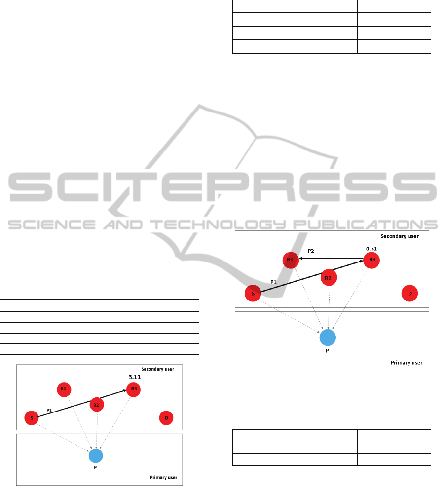
Without loss of generality, in our model we
assume the existence of maximum three relay nodes
(R1, R2 and R3) in the distance between the
secondary source (S) and the secondary destination
(D). Figure 3 illustrates the used system model with
different links between each relay, the source and
the destination. For paths: (S to D), (S to P), (R to
D), (S to P) and (R to P) the links are denoted by
,
,
,
, respectively, and the channel
coefficients are given as ℎ
,ℎ
,
ℎ
,ℎ
ℎ
respectively. Channel coefficients are considered as
Rayleigh fading in the form (Tran, 2013):
=|ℎ
|
,={0,1,2,3,4}
(1)
Ultimately,
is an exponential random variable
with a parameter
. To include the path-loss in
consideration, the parameter
can be modelled as
in (Duy, 2012) by:
=
(2)
β is the path-loss exponent which varies from 2 to 6,
and we consider it 3 (Tran, 2013).
We reflect the network topology on the X-Y plane,
and assume that the coordinates of the (S),(D),(
)
and (P) are (0,0),(1,0),(
,
) and (,)
respectively, where (0<X
,0<
) and (<1,
PECCS2015-5thInternationalConferenceonPervasiveandEmbeddedComputingandCommunicationSystems
110
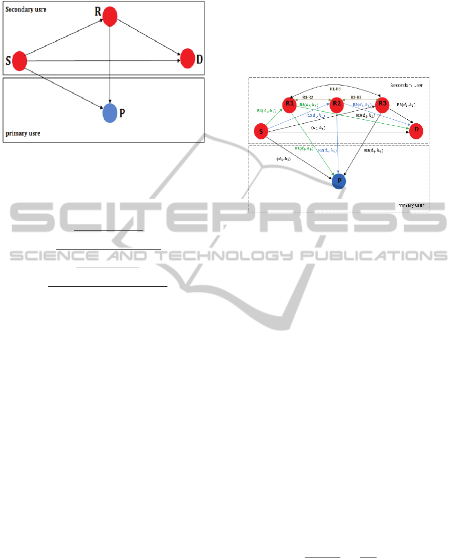
Figure 3: One Relay System Model.
<1), here for
, ∈{1,2,3} which represents the
different relay nodes see figure 4. The distances
between the system components are:
=1
(3)
=
(
)
+(
)
(4)
=
(1−
)
+(0−
)
(5)
=
()
+()
(6)
=
(−
)
+(−
)
(7)
In addition to the mentioned links, in this system
model we assume the existence of communication
links between the three relay nodes (R1-R2),(R2-R3)
and (R1-R3). The idea behind these connections is to
find the best relay path between the secondary
source and the secondary destination by creating
cooperation process between the relay nodes to
calculate the best path as shown in figure 4 and
explained in the next section.
3 PROTOCOL PROCEDURE
This paper adopts the one relay system protocol
calculation that has been applied in (Tran, 2013) as a
base point to enhance and develop choosing the best
path protocol from multiple relay node system.
The cooperative protocol (C) is the relay node
protocol that has been used in the relay technology.
This protocol works according to comparison
process for the signal to noise ratio (SNR) between
the direct path and the relay node path, the higher
SNR will be chosen as a best path. As we know the
(SNR) depends on the channel conditions and for
this paper the channels conditions had been assumed
randomly to be close to the reality as much as
possible.
Figure 4 shows the distances and the channels
coefficient for our system model. We assumed that
the source (S) and each relay node (R) have
knowledge in the channel information ℎ
and ℎ
so
that they have the ability to adapt their transmitted
power to satisfy the interference constraint at (P) as
(Guo, 2010).
Figure 4: Best Relay System Model.
Before the source transmits its data, a media
access control (MAC) layer operation which is
similar to the way in (Liu, 2006) is applied on the
system channels.
The source begins the process with a request-to-
send (RTS) message to the relay point and the
destination. Since the source is aware of the channel
informationℎ
, if is possible to add the parameters to
the (RTS) message. It is possible for the secondary
destination (D) to estimate the channel ℎ
and reacts
to the source by sending a clear-to-send (CTS)
message to it, and the destination includes the value
of ℎ
in this message. The relay node decodes the
(RTS) and (CTS) messages that have been received
from the secondary source to extract the needed
information while estimating ℎ
and ℎ
.
The relay node (R) makes a full conclusion to all
channels information; to calculate the (SNR) of the
relay links ℎ
and ℎ
and the direct link ℎ
in the
following stages:
Direct link is used (DL):
According to (Guo, 2010), the source adapts its
power with the allowable maximum transmitted
power
,
=
/
. And the (SNR) to this link
will be
=
/ℎ
/
/
ℎ
/
=
(8)
Where =
/
and
: is Gaussian noise
(assumed to be same at all receivers R and D).
Relay link is used (R):
In this paper we assumed that node has one antenna
BestPathSelectioninaMulti-RelayNodeSystemundertheConceptofCognitiveRadio
111

and each one will operate in half duplex mode and
the system used time division multiple access
(TDMA).
According to (Liu, 2006) the transmitted powers
of the relay link (S to R to D) are:
≤
/
and
≤
/
, where
and
are the transmitted
powers of (S) and (R), respectively.
The total transmitted power of (S) and (R) must
be under this condition:
+
=
=
/
(9)
The SNR for this relay link, decode and forward
relaying mode can be represented in a similar
fashion to (Laneman, 2004):
=
,
(10)
Depending on (Tran, 2013) we can formulate the
optimal
as in (11).
By comparing the SNR of both the direct link
and the relay link, the relay node detects whether if
it will cooperate with the source or not.
If
>
, then the relay will send to the
source and destination a not help to send message
(NHTS). In this case the source will use the direct
path between itself and the destination.
In the other cases the relay will send help to send
(HTS) message to inform that it will assist in the
source forwarding the data to the destination, and the
message includes the transmitted power of the
source
which was calculated in the (11), and the
source will adapt its power follows the
. (Tran,
2013) (Laneman, 2004).
By using MATLAB and from all these
calculations for each relay node a protocol had been
developed to establish a cooperative process
between the relay node to produce the best path for
the signal from the secondary source and the
secondary destination which is passing throw the
relay nodes that located in this distance. Where
during the procedure, (S) makes its calculations to
choose the best node and send the data to the best
relay selection in the first time slot. After that, the
best relay, which has received the data, will become
the new (S) in the system, so it will repeat the
previous calculations to detect the new best relay
selection in the rest of the system and send to the
new best relay selection the data in the second time
slot, etc.., until reaching (D).
In this paper, as we mentioned before, three relay
nodes system had been adopted that works on the
TDMA channel access and half duplex technique as
seen in Figure 4 which represents the general plan of
the best path selection system model.
The first time slot of the channel has been
reserved to the secondary source (S) to send the
information to the direct link or to the best relay
node which has been detected by the signalling
process that was applied on the whole system by the
source, after that the second time slot will be
reserved to the best relay node and it will be
considered as a new (S), after that the same process
of signalling was applied to detect the best relay
node from the rest of the nodes at the system or to
adopt the direct link as a best path between the new
(S) and (D), etc… till we get the best path.
We are dealing with each relay node and its
channels conditions in isolation from the other nodes
in the system. For each node in the first step we are
calculating the value of
, =
{
1,23
}
for
three relay nodes (
is SNR of the link between
S,R and D for each relay node) and
(SNR of the
direct link between S and D) and each value of
must exceed the two conditions : greater than the
value of
and greater than the
( the minimum
value of SNR that the receiver need it to detect the
signal) of the destination, to be considered as an
active relay node, or we define it by zero value. By
comparing the values of the
with the value of
the
, if any value of
is greater than
then the
node which has the greatest
has the ability to
work as a relay node to be the best relay selection
and the new secondary source in the same time, at
that point the second step will start and all the
previous calculations will be repeated on the rest of
nodes in the system and the direct link between the
new secondary source and the destination till we
find the best path, unless the value of
in the first
step will be the greatest value of SNR in the system
so the protocol will choose the direct path as the best
path. We repeated this process for all the relay nodes
with the channel conditions for each relay node path
and direct path.
=
(
+
)
;
+
<
=
(
+
)
,
=
(
+
)
;
+
≥
=
−
,
=
(11)
PECCS2015-5thInternationalConferenceonPervasiveandEmbeddedComputingandCommunicationSystems
112
4 SIMULATION RESULTS
As we mentioned before, by using MATLAB the
best path protocol had been created. In this part of
the paper we present examples of the way that the
protocol worked. Also, it presents the system
performance calculations which are based on some
variable have been taken in the consideration.
For the procedure of the best path selection
protocol, the work in this took a lot of cases of
implementing the Protocol on different relay nodes
points with different values of Q and different
positions for the primary user (P). For example:
Best path with PU at (0.5, 0.5) and=5:
In this example, we fixed the position of (P) at
(0.5,0.5), and applied the value of
=0.3, then
we chose multiple cases each one depended the relay
nodes positions R1(
,
), R2(
,
), and R3(
,
)
on (0.9,0.2) (0.75,0.1) (0.82,0), with 5 for the value
of .
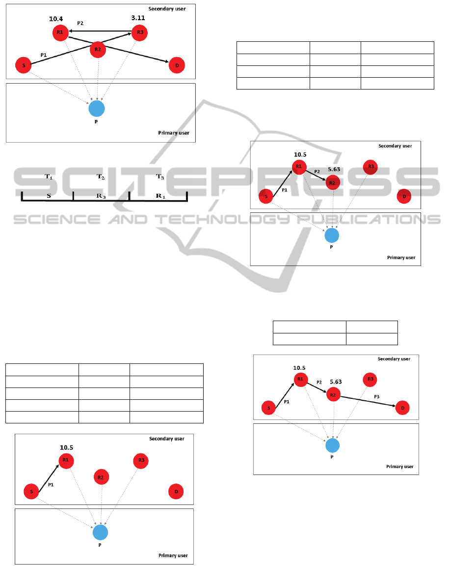
Step1: In this step the system made its calculation to
choose the best SNR, where it detected R3 as the
best relay node which can be seen in table 1. Figure
5 explains the first step operation.
Table 1: Step one for the path cases at (0.9, 0.2) (0.75,0.1)
(0.82,0).
Path
Case
S-R1 0 OFF
S-R2 0 OFF
S-R3 3.11 ON
S-D 0.54 OFF
Figure 5: First Step Choosing the Best Path.
Step2: In this stage, R1 has been detected as the best
relay node as shown in Figure 6 and table 2.
Step3: The last step showed the system choosing the
direct path between R1 and (D) to as the best path as
shown in figure 7 and table 3.
Table 2: Step two for the path cases at (0.9,0.2) (0.75,0.1)
(0.82,0).
Path
Case
R3-R1 10.46 ON
R3-R2 8.3 OFF
R1-D 3.8 OFF
The TDMA slots division for the previous case
in Figure 8, where the first time slot will be used by
the source and the second will go to R3 and the third
will go to R1.
As had been mentioned before, we used the
TDMA channel access with the half duplex
transmission technique. One of the disadvantages
that have been faced in our work is the delay,
because of our need to a single time slot for each
transmission process in the system, where we used
one time slot for the transmission of the secondary
source and one time slot for the transmission of each
relay node included in the calculations of choosing
the best path selection.
Figure 6: Second Step Choosing the Best Path.
Table 3: Step three for the path cases at (0.9, 0.2)
(0.75,0.1) (0.82,0).
Path
Case
R1-R2 0 OFF
R1-D 77.6 ON
To overcome this point, we can determine the
number of time slots to be used in the transmission
system, for example, if we depend on a system that
consists of multi relay nodes like a three relay node
system, we need four time slots when using the three
nodes as a relay node. For this, we minimized the
number of relay nodes that have been used in the
transmission system to reduce the delay of the
system, and this process was implemented by
BestPathSelectioninaMulti-RelayNodeSystemundertheConceptofCognitiveRadio
113
controlling the number of time slots that was used
for each transmission system.
Figure 7: Third Step Choosing the Best Path.
Figure 8: Time Slots Distribution.
For example, we took the case of the time slot
constraint with (P) position at (0.5, 0.5) and applied
the values of
=0.3 and Q=15dB and relay nodes
positions R1 at (0.7,-0.1), R2 at (0.85,-0.1) and R3 at
(0.9,0) and the process of creating the best path in
this form:
Step 1: R1 is the best relay node selection here, as
explained in figure 9 and table 4.
Table 4: Step one for the path cases at (0.7,-0.1) (0.85,-
0.1) (0.9,0).
Path
Case
S-R1 10.57 ON
S-R2 7.02 OFF
S-R3 0 OFF
S-D 5.62 OFF
Figure 9: First Step Choosing the Best Path.
Step2: In this step, R1 had been chosen by the
system as the best path, as figure 10 and table 5
shows.
Table 5: Step two for the path cases at (0.7,-0.1) (0.85,-
0.1) (0.9,0).
Path
Case
R1-R2 5.63 ON
R1-R3 0 OFF
R1-D 2.18 OFF
Step 3: The system chose the direct link, because
were bounding with two time slots as seen in figure
10 and table 6.
Figure 10: Second Step Choosing the Best Path.
Table 6: Step three for the path cases at (0.7,-0.1) (0.85,-
0.1) (0.9,0).
Path Case
R2-D ON
Figure 11: Third Step Choosing the Best Path (Obligatory
Step).
According to the time constraint, the time slots
division is described in figure 11.
This time slot constraint obligates the system to
work with two relay nodes even if the three nodes
have the ability to work as relay nodes to avoid the
delay in the system.
PECCS2015-5thInternationalConferenceonPervasiveandEmbeddedComputingandCommunicationSystems
114
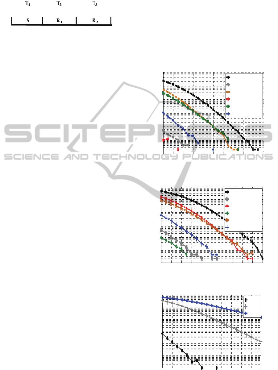
Figure 12: Time Slots Distribution.
In this part from the simulation results, we
calculated the outage performance of our proposed
protocol, where we proved that the best path system
performance is a huge breakthrough in improving
the performance of the system during the process
between the transmitter, the secondary source (S)
and the secondary destination (D).
Where we studied the outage probability of this
system in different relay nodes distribution with
different values of
.
We supposed that the secondary source (S) at the
(0, 0) position and the secondary destination (D) at
the (1,0) position, while the primary user location is
at (0.5,0.5).
For this protocol, we observed from the results
that the system performance behaves almost
randomly depending on the relationship between the
relay nodes, the primary user and the destination
positions. Overall, this protocol provides a great
performance on the path between the (S) and the
(D).
Outage probability calculations for
=0.5:
We applied 0.5 for the receiver
and from Figure
12 we observe that the best distribution for the relay
nodes is when all the relay nodes exist after the half
the distance between the secondary source and the
secondary destination, similar to the best relay
protocol case.
Outage probability calculations for
=1:
in this case was chosen to be 1. Figure 13
explains the outage probability of the system with
different relay nodes distribution sets.
In the final stage from the simulation results, the
paper presents a comparison between the outage
probability for the direct path system model, one
relay system model in (Tran, 2013) and the best path
system model.
We applied Monte Carlo simulation with 10
trails for different values of Q, ranging from 1 to 20
in each scenario, and we adopted =3. For the one
relay node system the authors in (Tran, 2013)
depended on the following positions for the
secondary source, the secondary destination and the
primary user (0,0), (1,0) and (0.5,0.5) respectively.
Also they adopted 0.5 as the value for the receiver
, and the relay node at the position (0.5,0).
Here we used the same values that have been
mentioned above in the one relay node protocol for
the secondary source, the secondary destination and
the primary user positions. Additionally, we fixed
the value of
to 0.5. The relay nodes positions in
the two proposed protocol are
R
(0.2,−0.2),R
(0.6,−0.1) and R
(0.9,−0.3).
Figure 14 presents the outage probability
compression results for the three system models as a
function of Q.
Figure 13: Outage Probability in Different Relay Nodes
Distributions.
Figure 14: Outage Probability in Different Relay Nodes
Distribution.
Figure 15: The Outage Probability Comparison.
0 2 4 6 8 10 12 14 16 18 20
10
-6
10
-5
10
-4
10
-3
10
-2
10
-1
10
0
(0.2,0.1)(0.3,0)(0.5,0.1)
(0.5,0)(0.75,0.1)(0.89,0.1)
(0.2,-0.1)(0.3,0)(0.5,-0.1)
(0.5,0)(0.75,-0.1)(0.89,-0.1)
(0.2,0.2)(0.6,0.1)(0.9,0.3)
(0.2,-0.2)(0.6,-0.1)(0.9,-0.3)
0 2 4 6 8 10 12 14 16 18 20
10
-6
10
-5
10
-4
10
-3
10
-2
10
-1
10
0
(0.2,0.1)(0.3,0)(0.5,0.1)
(0.5,0)(0.75,0.1)(0.89,0.1)
(0.2,-0.1))(0.3,0)(0.5,-0.1)
(0.5,0)(0.75,-0.1)(0.89,-0.1)
(0.2,0,2)(0.6,0.1)(0.9,0.3)
(0.2,-0.2)(0.6,-0.1)(0.9,-0.3)
0 2 4 6 8 10 12 14 16 18 20
10
-6
10
-5
10
-4
10
-3
10
-2
10
-1
10
0
Best Path
One Relay
Direct Link
Outage probability
Outage probability
Outage probability
BestPathSelectioninaMulti-RelayNodeSystemundertheConceptofCognitiveRadio
115

5 CONCLUSIONS
In this paper, we proposed a best path selection
system. The procedure is based on choosing the best
path between the secondary source and the
secondary destination by a cooperation process
between the relay nodes. Time delay is taken into
consideration in the case of best path protocol. A
solution is presented by using time constraint
protocol to overcome time delay. Numerical results
show a significant reduction in outage probability
when comparing with single relay node system, for
instance, a reduction from 10
to 10
is shown at
signal to noise ratio of 4.
REFERENCES
Goldsmith, A., August 2005. Wireless communication.
Cambridge University Press.
Mikio, L., Hideaki, T., and Satoshi, N., September 2010.
Relay technology in LTE advance. NTT DOCOMO
technical journal, VOL.12, NO.2.
Klaus, D., 2010. In-band Relays for Next Generation
Communication Systems. Aalto University School of
Science and Technology Department of Signal
Processing and Acoustics.
Juncheng, J., Jin, Z., and Qian, Z., 2009. Cooperative
Relay for Cognitive Radio Networks. INFOCOM
2009, IEEE.
Tran, T., Duy, and Hyung-Yun, K., 2013. Adaptive
Cooperative Decode-and-Forward Transmission with
Power Allocation under Interference Constrain.
Springer US, online ISSN: 1572-834X.
Duy, T., Kong, H., 2012. Performance Analysis of Two-
Way Hybrid Decode-and-Amplify Relaying Scheme
with Relay Selection for Secondary Spectrum Access.
Wireless Personal Communications, online first.
Guo, Y., Kang, G., Zhang, N., Zhou, W., and Zhang, P.,
January 2010. Outage performance of relay assisted
cognitive-radio system under spectrum-sharing
constraints. IEEE Electronics Letters,
Volume:46, Issue: 2.
Liu, P., Tao, Z., Lin, Z., Erkip, E., and Panwar, S., 2006.
Cooperative wireless communications: a cross-layer
approach. IEEE Wireless Communication,13, 84 - 92.
Laneman, J., Tse, D., and Wornell, G., 2004. Cooperative
diversity in wireless networks: Efficient protocols and
outage behavior. IEEE Trans. on Inform. Theory, 50,
pp. 3062 - 3080.
Rahul, C., and Gundal, S., March 2013. Cognitive radio
networks. International Journal of Electronics,
Communication & Instrumentation Engineering
Research and Development (IJECIERD), Vol. 3, Issue
1.
Ding, H., Ge, J., Da Costa, B., and Zhuoqin J., 2011.
Asymptotic Analysis of Cooperative Diversity
Systems with Relay Selection in a Spectrum-Sharing
Scenario. IEEE Transactions on Vehicular
Technology, 60, pp. 457-472.
Duong, T., Da Costa, M., Elkashlan, M., and Bao, V.,
2012. Cognitive Amplify-and-Forward Relay
Networks over Nakagami-m Fading. IEEE
Transactions on Vehicular Technology, 61, pp. 2368-
2374.
Han, Y., Ting, S., 2009. Cooperative Decode-and-Forward
Relaying for Secondary Spectrum Access. IEEE
Transaction on Wireless Communication, 8, pp. 4945-
4950.
PECCS2015-5thInternationalConferenceonPervasiveandEmbeddedComputingandCommunicationSystems
116
