Combined Bilateral Filter for Enhanced Real-time Upsampling

of Depth Images

Oliver Wasenm

uller, Gabriele Bleser and Didier Stricker

Germany Research Center for Artiﬁcial Intelligence (DFKI), Trippstadter Str. 122, Kaiserslautern, Germany

Keywords:

Depth Image, Upsampling, Joint Bilateral Filter, Texture Copying, Depth Discontinuity, Sensor Fusion.

Abstract:

Highly accurate depth images at video frame rate are required in many areas of computer vision, such as 3D

reconstruction, 3D video capturing or manufacturing. Nowadays low cost depth cameras, which deliver a high

frame rate, are widely spread but suffer from a high level of noise and a low resolution. Thus, a sophisticated

real time upsampling algorithm is strongly required. In this paper we propose a new sensor fusion approach

called Combined Bilateral Filter (CBF) together with the new Depth Discontinuity Preservation (DDP) post

processing, which combine the information of a depth and a color sensor. Thereby we especially focus on

two drawbacks that are common in related algorithms namely texture copying and upsampling without depth

discontinuity preservation. The output of our algorithm is a higher resolution depth image with essentially

reduced noise, no aliasing effects, no texture copying and very sharply preserved edges. In a ground truth

comparison our algorithm was able to reduce the mean error up to 73% within around 30ms. Furthermore, we

compare our method against other state of the art algorithms and obtain superior results.

1 INTRODUCTION

Within recent years low-cost depth cameras are

widely spread. These cameras are able to measure the

distance from the camera to an object for each pixel

at video frame rate. There are two common technolo-

gies to measure depth. Time-of-Flight (ToF) cameras,

such as the SwissRanger or the Microsoft Kinect v2,

emit light and measure the time the light takes to re-

turn to the sensor. Structured light cameras, such as

the Microsoft Kinect v1 or the Occipital Structure,

project a pattern into the scene and capture the local

disparity of the pattern in the image. In all these cam-

eras high speed and low price are accompanied by low

resolution (e.g. Kinect v2: 512 × 484px) and a high

level of noise. However, their application areas, such

as 3D reconstruction of non-rigid objects, 3D video

capturing or manufacturing, require both high qual-

ity depth estimates and fast capturing. High-end de-

vices, such as laser scanners, provide extremely ac-

curate depth measures, but are usually expensive and

only able to measure a single point at a time. Thus,

a sophisticated ﬁlter algorithm to increase the resolu-

tion and decrease the noise level of depth images in

real-time is strongly required.

In this paper we propose an enhanced real-time

iterative upsampling, which we call Combined Bilat-

eral Filter (CBF). Our new algorithm is based on a

fusion of depth and color sensor with the principle

of Joint Bilateral Filtering (JBF) (Kopf et al., 2007).

Such algorithms take as an input a low resolution

and noisy depth image together with a high resolu-

tion color image as e.g. Kinect produces it. They

process the two images to a high resolution noise-

reduced depth image as shown in Figure 1. Thereby

we especially focus on two drawbacks that are com-

mon in JBF based algorithms namely texture copy-

ing and no depth discontinuity preservation. Texture

copying (see Figure 5(k)) is an artifact that occurs

when textures from the color image are transferred

into geometric patterns that appear in the upsampled

depth image. Our proposed ﬁlter algorithm is a new

combination of a traditional bilateral ﬁlter with a JBF

to avoid texture copying. The new Depth Discontinu-

ity Preservation (DDP) post processing step prohibits

wrong depth estimates close to edges (see Figure 4),

which occur in many bilateral ﬁlters. The remainder

of this paper is organized as follows: Section 2 gives

an overview of existing methods for depth image up-

sampling. The proposed CBF algorithm and the DDP

post processing are motivated and explained in detail

in Section 3, while they are evaluated regarding qual-

ity and runtime in Section 4. The work is concluded

in Section 5.

Wasenmüller O., Bleser G. and Stricker D..

Combined Bilateral Filter for Enhanced Real-time Upsampling of Depth Images.

DOI: 10.5220/0005234800050012

In Proceedings of the 10th International Conference on Computer Vision Theory and Applications (VISAPP-2015), pages 5-12

ISBN: 978-989-758-089-5

 2015 SCITEPRESS (Science and Technology Publications, Lda.)

(a) (b) (c)

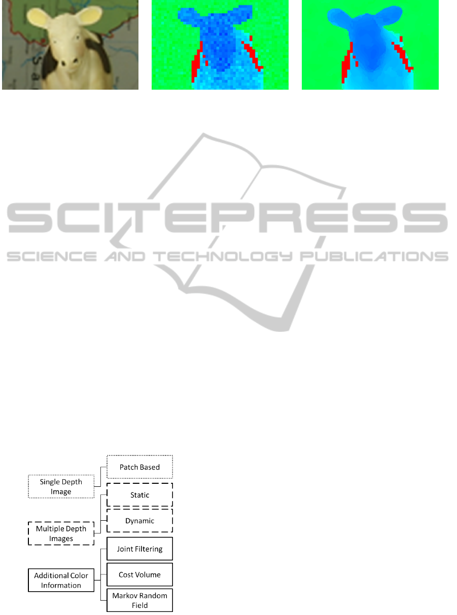
Figure 1: Proposed ﬁlter. (a) Color input image. (b) Depth input image. (c) Final result: signiﬁcantly reduced noise,

no aliasing effects, no texture copying, very sharply preserved edges and a higher resolution. Baby3 dataset taken from

(Scharstein and Szeliski, 2003). Red pixels have no depth value.

2 RELATED WORK

Depth image upsampling is a well-known problem in

the literature and its currently established solutions

can be subdivided into three main categories. A rough

classiﬁcation is depicted in Figure 2.

In the ﬁrst main category the upsampling is based

on one single depth image. Besides simple upsam-

pling, which is not considered here, this includes

methods that apply machine learning approaches like

for example in (Aodha et al., 2012). Additional infor-

mation is here provided via training patches with pairs

of low and high resolution depth images that show dif-

ferent scenes. After training the patches an upsampled

image can be computed based on the training data.

However, the training dataset needs to be represen-

tative, whereas runtime grows with the database size.

Thus, a patch based approach is not applicable for real

time upsampling.

In the second main category the upsampling is

based on multiple depth images, which were captured

either from a moving camera or multiple displaced

cameras. This requires to register the input images

Figure 2: A rough classiﬁcation of current methods for

depth image upsampling.

and to ﬁnd a suitable way to combine them to an up-

sampled image. These methods differ in the ability

to cope with displacement. Thus, a classiﬁcation into

static methods with small displacement (e.g. (Schuon

et al., 2009)) and dynamic methods with large dis-

placement (e.g. (Cui et al., 2010)) is reasonable.

However, none of these methods is able to process

depth images in real time and thus they are not suit-

able for our purpose.

In the third main category the upsampling is based

on one depth image and one simultaneously captured

color image. The methods are based on the assump-

tion of coherent depth and color discontinuity, mean-

ing that edges in the color image coincide with edges

in the depth image and vice versa.

One approach for using color information in depth

images is a Markov Random Field (MRF) as proposed

in (Diebel and Thrun, 2005). Therefore, they deﬁne

the posterior probability of the upsampled depth im-

age as a MRF and optimize for the maximum a pos-

teriori solution. However, this approach suffers from

texture copying and high calculation time.

Another approach to use color information in

depth images is a cost volume approach as proposed

in (Yang et al., 2007). This is based on minimiza-

tion of costs in a volume with different depth hypothe-

ses. After initial construction of the volume, a ﬁlter is

applied on each depth hypothesis and for each pixel

the depth value with lowest cost is chosen. The ﬁlter

is one of the crucial points in this method and often

realized by an edge preserving ﬁlter. This principle

suffers also from texture copying, but preserves sharp

edges very well. However, it has a high complexity,

since the ﬁlter must be applied to each single depth

hypothesis. Thus, it has a high calculation time and is

not suitable for our purpose.

The last common approach to use color informa-

tion in depth images is Joint Bilateral Filtering (JBF).

The basic idea comes from 2D image ﬁltering, where

the bilateral ﬁlter (BF) for smoothing images and at

the same time preserving edges was introduced in

VISAPP2015-InternationalConferenceonComputerVisionTheoryandApplications

(Tomasi and Manduchi, 1998). The key idea of this

ﬁlter is that the inﬂuence of a pixel in the calcula-

tion of another pixel does not only depend on spatial

neighborhood but also on similar color values. The

BF is computed for a pixel p from the input image I

in a neighborhood N around p by

Tomasi

(I)

∑

q∈N

p,q

∑

q∈N

p,q

· I

(1)

with W

p,q

= G

(p −q)G

− I

where W

p,q

is a weighting factor, G

is the spatial

ﬁlter kernel and G

is the range ﬁlter kernel. The

spatial ﬁlter kernel G

is a Gaussian with variance σ

centered at the pixel p and decreases the inﬂuence of

distant pixels q. On the other hand the range ﬁlter ker-

nel G

is a Gaussian with variance σ

that decreases

the inﬂuence of pixels q with distant color I

to I

This idea was extended in (Kopf et al., 2007) to the

JBF, where a depth image D is ﬁltered with the guid-

ance of a color image I. A pixel in the depth image is

then inﬂuenced by neighboring pixels depending on

their distance and the difference of the corresponding

color values. The JBF can be computed for a pixel p

from the depth image D and the color image I by

JBF

Kop f

(D, I)

∑

q∈N

p,q

∑

q∈N

p,q

· D

(2)

with W

p,q

= G

(p − q)G

− I

The main assumption here is again coherent depth

and color discontinuity leading to texture copying in

regions, which are both ﬂat and textured. This prob-

lem was addressed in some related work like e.g. in

(Kim et al., 2011) by an extension of the JBF. They

add a blending function α to the JBF in order to con-

trol the inﬂuence of the spatial kernel G

and the

range kernel G

. The idea is to differentiate two

cases and ﬁlter pixels of ﬂat areas with the spatial ker-

nel, in order to avoid texture copying, while pixels of

edge areas are ﬁltered with the range kernel. The ﬁl-

ter can then be computed for a pixel p from the depth

image D and the color image I by

JBF

Kim

(D, I)

∑

q∈N

p,q

·W

p,q

(3)

with W

p,q

∑

q∈N

[(1 − α(∆

))G

(p − q) +

α(∆

− I

)]D

and α (∆

) =

1 + e

−ε(∆

−τ)

where W

p,q

is a weighting factor. In the considered

neighborhood N the difference between the maximum

and minimum depth value is ∆

, whereas ε and τ are

constants. The min-max difference τ determines at

which value the blending interval shall be centered,

whereas ε controls the width of the transition area

between the two cases. This method avoids texture

copying quite well but performs poorly in edge re-

gions (Figure 6).

3 METHOD

Our proposed ﬁlter is able to iteratively upsample a

low resolution and noisy depth image in real time.

Therefore, we use a new so-called Combined Bilat-

eral Filter (CBF, see Section 3.1) composed of a Joint

Bilateral Filter (JBF) and traditional Bilateral Filter

(BF). With this combination the ﬁlter avoids texture

copying. The new Depth Discontinuity Preservation

(DDP) post processing step in Section 3.2 prohibits

wrong depth estimates close to edges, which occur

in many bilateral ﬁlters. The whole iterative ﬁltering

process is explained in Section 3.3. An overview of

our ﬁlter is given in Figure 3, while its details are out-

lined below.

3.1 Combined Bilateral Filter (CBF)

The proposed CBF is driven by the observation that

the JBF delivers good results for edge areas in depth

images, but performs poorly in ﬂat depth image re-

gions by introducing artefacts like texture copying.

These artefacts are mainly caused by the inﬂuence of

the color information. Thus, we ﬁlter the depth image

in ﬂat regions without any guidance of color informa-

tion by a traditional BF (see Equation 1). Note, in

contrast to the ﬁlter of (Kim et al., 2011) in Equa-

tion 3 we still ﬁlter by an edge preserving ﬁlter in ﬂat

areas. This enables us to preserve also ﬁne depth dis-

continuities in (almost) ﬂat regions.

The crucial point is to determine the type of re-

gion (ﬂat or edge) in a depth image for a given point.

A straight forward approach with an edge detection

algorithm like e.g. (Canny, 1986) as preprocessing is

not suitable here, because our ﬁlter should run in real

time. Thus, we need to determine the type of region

while ﬁltering.

In our approach two ﬁlters - the BF and the JBF -

are applied in parallel for a given pixel p. The type of

region is then estimated based on the difference ∆

these two ﬁlter results with

∆

= |JBF(D, I)

− BF(D)

|. (4)

The difference ∆

is low in ﬂat regions and high in

edge regions. Thus, the CBF can be computed for a

CombinedBilateralFilterforEnhancedReal-timeUpsamplingofDepthImages

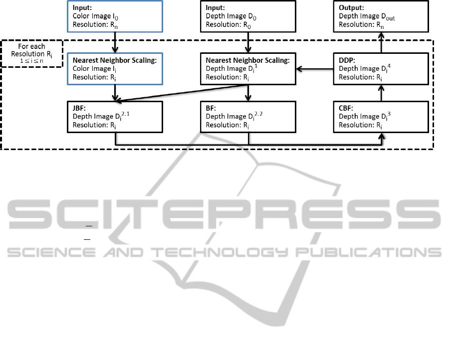
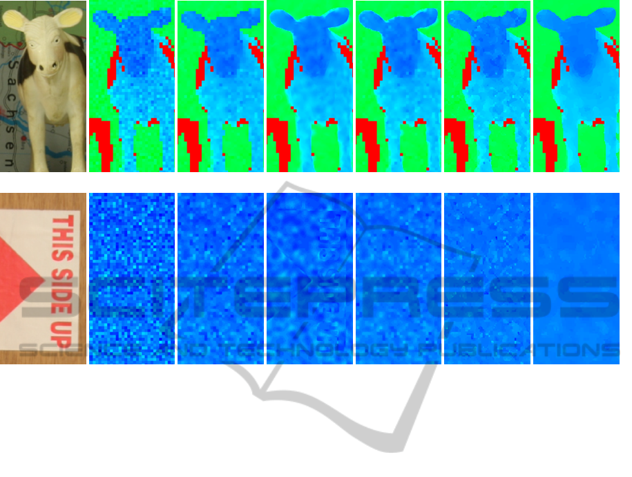
Figure 3: Schematic overview of proposed depth image upsampling ﬁlter.

pixel p from the depth image D and the color image I

CBF(D, I)











JBF(D, I)

, ∆

> s

cos



∆



BF(D)

sin



∆



JBF(D, I)

, ∆

≤ s

, (5)

where s is a manually chosen threshold to determine

above which value of ∆

only the JBF is used any-

more. With the decision to use sine and cosine re-

spectively as blending function a normalization is not

necessary, since ∀x : sin

x + cos

x = 1.

3.2 Depth Discontinuity Preservation

(DDP)

The CBF is an edge preserving ﬁlter, since it is com-

posed of the two edge preserving ﬁlters BF and JBF.

However, after ﬁltering ﬁne blur still remains around

edges in the depth image just as in the BF and JBF.

For 2D images, where the bilateral ﬁltering concept

comes from, this has not a high impact, since ﬁne blur

around edges still looks appealing from a visual point

of view. Certainly, ﬁne blur around edges in depth im-

ages has a high impact as shown in Figure 4. If a depth

sensor captures two distant but overlapping planes, it

captures (nearly) no pixels between these two planes.

However, by ﬁltering with a JBF or a BF a transition

consisting of pixels between the two planes is created.

These pixels are of course substantially wrong, since

in reality there is no connection between the planes

and also the depth sensor did not capture any connec-

tion. This error occurs in many existing bilateral ﬁlter

based depth image ﬁltering algorithms.

Thus, in this paper we propose a new post pro-

cessing ﬁlter called Depth Discontinuity Preservation

(DDP) to avoid depth transitions between different

depth levels. The goal is to adjust wrong ﬁlter results

by shifting pixels to the correct depth level. The idea

of DDP is that the edge preserving ﬁlter should only

output a pixel p, whose depth value was already exist-

ing before ﬁltering in a small neighborhood N around

p. This idea is similar to a median ﬁlter, but in con-

trast DDP retains the edge preserving property of the

input ﬁlter like e.g. the CBF. More formally, DDP

ﬁlters a pixel p for a raw depth image D and a CBF

result (cf. Equation 5) by

DDP(D,CBF)

CBF



j ∈ N;∀k ∈ N :

kCBF

− D

k ≤ kCBF

− D

, (6)

where N is a small neighborhood around p. The effect

of DDP is discussed in Section 4 (see Figure 4).

3.3 Filtering Process

Our ﬁlter (see Figure 3) takes as an input a color Im-

age I

with a high resolution R

and a depth image

with a low resolution R

. The goal is to increase

the resolution of D

from R

to R

. Therefore, we use

an iterative procedure with n iterations. Unlike other

methods we do not directly upsample D

from R

and ﬁlter afterwards several times on the highest

resolution, since ﬁltering on high resolutions is time

consuming. Our method converges to resolution R

each iteration in a linear way.

In the i-th iteration both the color image I

and the

depth image D

i−1

are scaled to resolution R

resulting

in I

and D

respectively. The BF (Equation 1) and

the JBF (Equation 2) are then applied to I

and D

required for our CBF (Equation 5). The output of the

CBF is the depth image D

, which is reﬁned by our

DDP (Equation 6) ﬁlter to D

. If the ﬁnal resolution

is reached (i = n) the depth image D

is the ﬁnal result

out

, otherwise the next iteration starts. The effects of

each step are illustrated in Figure 5 and are reviewed

in Section 4.

VISAPP2015-InternationalConferenceonComputerVisionTheoryandApplications

(a) (b) (c) (d)

(e) (f) (g) (h)

Figure 4: Depth Discontinuity Preservation (DDP). (a),(e): input depth image. (b),(f): joint bilateral ﬁlter (JBF) or combined

bilateral ﬁlter (CBF). (c),(g): JBF or CBF with DDP postprocessing. (d),(h): ground truth. Top row: 2D depth image. Bottom

row: depth image in 3D view. Wood2 dataset taken from (Scharstein and Szeliski, 2003).

4 EVALUATION

In this section we evaluate our CBF algorithm. There-

fore, we ﬁrst explain our evaluation setup in Section

4.1. In a second step we evaluate our CBF algorithm

from a visual point of view in Section 4.2. At the end

we compare in Section 4.3 our CBF algorithm against

ground truth data and related algorithms.

4.1 Evaluation Setup

The evaluation of depth images is not trivial, since

it is hard to produce ground truth data. Thus, we

used - like many other authors - the disparity images

of the stereo datasets of Middlebury (Scharstein and

Szeliski, 2003) in the evaluation of our algorithm. A

disparity image can also be seen as a depth image, be-

cause depth and disparity are directly related. Hence,

the disparity images with a resolution of 1282×1110

are used as ground truth data.

For the simulation of depth sensor data we down-

sample the resolution by factor 4, since real depth

data has a resolution in this range. To simulate the

depth sensors noise we add a Gaussian noise with a

standard deviation of 4 to the downsampled image.

The downsampled and noisy depth image serves then

as an input for both our developed and competitive

depth image upsampling algorithms. In the ground

truth comparisons of this section we compare the out-

put of a given ﬁlter against the raw depth image. To

demonstrate the effects of depth image upsampling

algorithms we distinguish between ﬂat and edge ar-

eas. The edges are detected by a Canny edge detec-

tor (Canny, 1986) and then dilated to cover the whole

edge area. The ﬂat areas are the complement of the

edge areas. For the quantitative evaluation we choose

two measures: For a depth image D and ground truth

image G with n pixels the Mean Error (ME) can be

estimated by

ME(D, G) =

∑

i=1

− G

k (7)

and the Error Rate (ER) by

ER(D, G) =

∑

i=1

, ∀p

: kD

− G

k > 2. (8)

The ER gives the percentage of pixels, which have

an error greater than 2. The quality of both our CBF

algorithm and competitive algorithms depends on the

choice of the corresponding parameters. We chose

the parameters of Table 1 empirically in several tests

to achieve the best results for each algorithm.

Table 1: Parameters of evaluated algorithms.

|N| σ

s ε τ

CBF + DDP 49 3 2 18 - -

JBF

Kop f

49 3 2 - - -

JBF

Kim

49 3 0.5 - 15 0.5

Cost Volume 49 3 3 - - -

4.2 Qualitative Evaluation

In this section we qualitatively evaluate the effects of

our new ﬁlter. Therefore, Figure 5 shows the resulting

depth image after each single ﬁltering step. The top

row (Figure 5 (a)-(g)) demonstrates the effects of edge

CombinedBilateralFilterforEnhancedReal-timeUpsamplingofDepthImages

(a) I

(b) D

2.2

(d) D

2.1

(e) D

(f) D

(g) D

(h) I

(i) D

(j) D

2.2

(k) D

2.1

(l) D

(m) D

(n) D

Figure 5: Illustration of each step in our ﬁlter for two exemplary zoomed datasets. (a),(h): input color image. (b),(i): input

depth image. (c),(j): bilateral ﬁlter. (d),(k): joint bilateral ﬁlter. (e),(l): combined bilateral ﬁlter (CBF). (f),(m): depth

discontinuity preservation (DDP). (g),(n): ﬁnal result after two iterations. Top row: Baby3 dataset. Bottom row: Wood2

dataset. Each taken from (Scharstein and Szeliski, 2003). Red pixels have no depth value.

preserving ﬁltering while removing noise, whereas

the bottom row (Figure 5 (h)-(n)) illustrates the ﬁl-

tering of a ﬂat and textured region. The ﬁrst column

shows the high resolution color input image I

and the

second column depicts the low resolution depth input

image D

with lots of noise.

After ﬁltering with a BF the noise in D

2.2

is re-

duced but still clearly visible. The edges around the

ears show aliasing effects, but also no texture was

copied into the depth image. In contrast, the JBF re-

duces much more noise in D

2.1

and also aliasing at

the edges of the ear is not visible anymore. However,

texture was copied into the depth image as visible in

Figure 5 (k). Here, the 3D structure contains the bor-

ders of the characters in Figure 5 (h), the triangle and

the rectangle. Furthermore, around the edges ﬁne blue

is visible.

Our CBF combines the results of BF and JBF

as well as their particular advantages. The resulting

depth image D

has a lower level of noise, shows

no aliasing effects and contains no texture in its 3D

structure. There is only one drawback left: around

the depth discontinuities, e.g. at the ears, ﬁne blur is

still visible.

Our DDP post processing in D

removes the ﬁne

blur in edge regions and still aliasing effects are

avoided. This is even better visible in 3D in Figure

4. Without DDP a non-existing transition between

the two distant depth levels is introduced, whereas

with DDP this connection is completely corrected.

Note, the wrong pixels in the transition area are not

removed but corrected in their position. However, the

DDP slightly reduces the effect of smooth ﬁltering in

ﬂat regions (Figure 5 (m)). This is due to the fact

that DDP outputs only values, which are present in a

neighborhood and these values must not be optimal

for smoothing, especially in ﬂat regions.

In our evaluation setup the whole ﬁlter runs two

iterations - each doubling the resolution - to achieve

the ﬁnal resolution. The output D

out

is a high reso-

lution depth image with essentially reduced noise, no

aliasing effects, no texture copying and very sharply

preserved edges.

4.3 Quantitative Evaluation

After qualitatively evaluating our results in the previ-

ous section, we quantify the quality of our algorithm

in this section. Therefore, we conduct a ground truth

comparison as speciﬁed in Section 4.1 and compare

VISAPP2015-InternationalConferenceonComputerVisionTheoryandApplications

(a) Whole Image.

(b) Edge Regions.

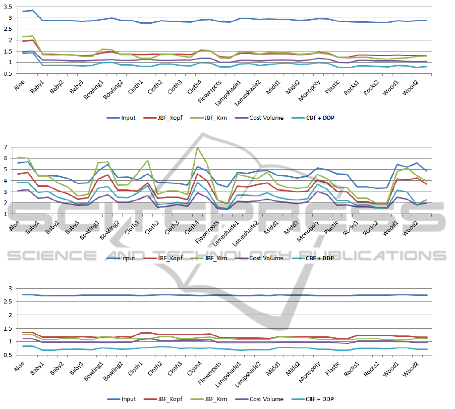
Figure 6: Mean Error (see Equation 7) for all datasets of (Scharstein and Szeliski, 2003) in denoted regions.

the results with competitive algorithms.

Figure 6 shows the Mean Error (ME) for three

kinds of image regions of all 42 datasets of

(Scharstein and Szeliski, 2003). In the whole image

both JBF

Kop f

and JBF

Kim

can halve the ME compared

to the input, whereas the Cost Volume approach re-

duces the ME by around 60%. Our algorithm on the

other hand is able to reduce the ME by up to 73%.

In edge regions our algorithm (ME ≈ 2.5) performs

slightly worse than the Cost Volume (ME ≈ 2.1),

but still better than JBF

Kop f

(ME ≈ 3.2) and JBF

Kim

(ME ≈ 3.9). However, the Cost Volume has a high

complexity, meaning that our algorithm is the best

performing of the real-time capable algorithms. In ﬂat

regions, which contain most pixels, our algorithm is

superior compared to all other evaluated algorithms.

In Table 2 the Error Rate (ER) in % is used as quality

measure and the results are similar to the ME.

To enable the real-time performance of our CBF

ﬁlter including the DDP post processing we ported

our code to the GPU. Since the GPU offers a fast par-

allel computing and our algorithms are calculated for

each pixel independently, we achieve without exces-

sive GPU optimization an performance gain of up to

2000× compared to the CPU. In our evaluation setup

(see Section 4.1) we are able to upsample a depth im-

age with our CBF including DDP within around 30

milliseconds on a NVIDIA GeForce GTX 660 Ti. The

parallel computation of both the BF and the JBF is

very effective and takes in our implementation only

around 10% more calculation time than one single ﬁl-

ter. As long as the GPU provides enough parallel pro-

CombinedBilateralFilterforEnhancedReal-timeUpsamplingofDepthImages

Table 2: Error Rate (see Equation 8) in % for a representative selection of datasets of (Scharstein and Szeliski, 2003) in

denoted regions.

Dataset Input JBF

Kop f

JBF

Kim

Cost Volume CBF + DDP

all edge ﬂat all edge ﬂat all edge ﬂat all edge ﬂat all edge ﬂat

Aloe 46.4 49.7 45.7 18.2 35.1 14.3 14.2 44.4 7.2 9.2 14.8 7.9 9.3 27.4 5.2

Baby3 45.9 47.6 45.7 11.8 24.6 10.1 5.9 25.4 3.4 6.2 13.6 5.2 5.0 17.2 3.5

Bowling2 45.7 48.4 45.4 11.7 26.6 10.2 5.7 26.2 3.6 6.0 12.5 5.3 4.9 19.8 3.3

Cloth4 45.7 49.4 45.4 14.3 33.4 12.7 7.0 44.9 4.1 7.6 14.7 7.0 5.4 30.7 3.4

Flowerpots 45.6 46.9 45.5 10.3 21.4 9.2 4.5 18.6 3.1 5.2 10.7 4.6 3.8 14.0 2.8

Midd2 45.9 48.2 45.6 11.5 25.8 10.0 6.9 26.2 4.9 5.8 10.5 5.4 5.8 18.2 4.5

Rocks1 45.9 48.9 45.5 12.9 24.3 11.7 5.8 25.3 3.7 6.9 14.7 6.1 4.7 17.3 3.3

Wood2 45.6 46.7 45.6 10.5 24.8 9.9 3.8 24.4 2.8 5.2 8.8 5.0 3.2 14.9 2.6

cessing units, the processing time does not increase

for higher resolutions. However, in general the pro-

cessing time is linear to the resolution and quadratic to

the radius of the neighborhood N around a processed

pixel.

5 CONCLUSION

The proposed Combined Bilateral Filter (CBF) to-

gether with the new Depth Discontinuity Preservation

(DDP) post processing is able to upsample a noisy

depth image in real time with the guidance of a color

image. Our CBF ﬁlter explicitly avoids texture copy-

ing and the DDP preserves edges very sharply. The

output of our algorithm is a high resolution depth

image with essentially reduced noise and no alias-

ing effects. Compared to existing algorithms such

as JBF

Kop f

(Kopf et al., 2007), JBF

Kim

(Kim et al.,

2011) and Cost Volume (Yang et al., 2007) we over-

all achieve superior results with our algorithm. Our

algorithm is able to reduce the mean error within

around 30ms up to 73% in a ground truth comparison.

Furthermore, our algorithm can be used as a stand-

alone pre processing for existing algorithms whenever

depth images are needed as an input.

ACKNOWLEDGEMENTS

This work was partially funded by the Federal Min-

istry of Education and Reseach (Germany) in the

context of the projects ARVIDA (01IM13001J) and

DENSITY (01IW12001). Furthermore, we want to

thank Vladislav Golyanik for his advise in GPU pro-

gramming.

REFERENCES

Aodha, O. M., Campbell, N. D., Nair, A., and Brostow,

G. J. (2012). Patch based synthesis for single depth

image super-resolution. In Proceedings of the Euro-

pean Conference on Computer Vision (ECCV), pages

71–84. Springer.

Canny, J. (1986). A computational approach to edge detec-

tion. In Transactions on Pattern Analysis and Machine

Intelligence (PAMI), volume 6, pages 679–698. IEEE.

Cui, Y., Schuon, S., Chan, D., Thrun, S., and Theobalt, C.

(2010). 3D shape scanning with a time-of-ﬂight cam-

era. In Conference on Computer Vision and Pattern

Recognition (CVPR), pages 1173–1180. IEEE.

Diebel, J. and Thrun, S. (2005). An application of markov

random ﬁelds to range sensing. In Advances in neural

information processing systems (NIPS), pages 291–

298. NIPS.

Kim, C., Yu, H., and Yang, G. (2011). Depth super resolu-

tion using bilateral ﬁlter. In International Congress on

Image and Signal Processing (CISP), volume 2, pages

1067–1071. IEEE.

Kopf, J., Cohen, M. F., Lischinski, D., and Uyttendaele, M.

(2007). Joint bilateral upsampling. In ACM Transac-

tions on Graphics (TOG), volume 26, page 96. ACM.

Scharstein, D. and Szeliski, R. (2003). High-accuracy

stereo depth maps using structured light. In Con-

ference on Computer Vision and Pattern Recognition

(CVPR), volume 1, pages 1–195. IEEE.

Schuon, S., Theobalt, C., Davis, J., and Thrun, S. (2009).

LidarBoost: Depth superresolution for ToF 3D shape

scanning. In Conference on Computer Vision and Pat-

tern Recognition (CVPR), pages 343–350. IEEE.

Tomasi, C. and Manduchi, R. (1998). Bilateral ﬁltering for

gray and color images. In International Conference

on Computer Vision (ICCV), pages 839–846. IEEE.

Yang, Q., Yang, R., Davis, J., and Nist

er, D. (2007). Spatial-

depth super resolution for range images. In Con-

ference on Computer Vision and Pattern Recognition

(CVPR), pages 1–8. IEEE.

VISAPP2015-InternationalConferenceonComputerVisionTheoryandApplications