A Parametric Space Approach to the Computation of Multi-scale

Geometric Features

Anthousis Andreadis, Georgios Papaioannou and Pavlos Mavridis

Department of Informatics, Athens University of Economics and Busines, Athens, Greece

Keywords:

Geometric features, Parametric space, Mesh geometry.

Abstract:

In this paper we present a novel generic method for the fast and accurate computation of geometric features

at multiple scales. The presented method works on arbitrarily complex models and operates in the parametric

space. The majority of the existing methods compute local features directly on the geometric representation

of the model. Our approach decouples the computational complexity from the underlying geometry and in

contrast to other parametric space methods, it is not restricted to a speciﬁc feature or parameterization of the

surface. We show that the method performs accurately and at interactive rates, even for large feature areas of

support, rendering the method suitable for animated shapes.

1 INTRODUCTION

Geometric features, like curvature and surface rough-

ness, are central to demanding computations in a wide

range of applications, including object retrieval and

registration, texture synthesis, stylized rendering and

many more. The computation of these fundamental

metrics is usually performed by CPU algorithms that

operate on a discrete polygonal representation of a

continuous surface. These metrics can be precom-

puted for static meshes, but their fast computation

even for moderately large or dynamic meshes, is chal-

lenging.

In this paper we focus on the general class of met-

rics with ﬁnite local support, whose computation de-

pends on the local neighborhood of an arbitrary point

p on the object’s surface. Robustness in the presence

of noise is achieved through multi-scale computation

of the features (Yang et al., 2006). To this end, a

data structure that encodes the adjacency information

is required, in order to efﬁciently locate the neigh-

boring points on a surface. This is especially true

for algorithms that operate on meshes. The compu-

tational complexity of such an object-space approach

is directly proportional to the geometric density and

quadratic with respect to the extent (i.e. radius) of

the local feature support. Despite the fact that com-

puting the metric for independent surface points is an

inherently parallel task, the use of complex data struc-

tures for storing the adjacency information prevents a

trivial and efﬁcient mapping of these computations to

Figure 1: a) ”Lucy” model (200K) colorized with mean cur-

vature, computed in 49ms, b) geometry (position) buffer

(normalized for visualization), c) surface normal buffer, d)

polygon chart identiﬁers (colorized for clarity) along with

the adjacent chart identiﬁers on border pixels, e) mean cur-

vature in parametric space (colorized for visualization).

massively parallel stream processors, like commod-

ity GPUs, at an arbitrary neighborhood scale. For

these reasons, real-time computation is often limited

to meshes with relatively low geometric complexity

and 1-ring vertex neighborhoods(Grifﬁn et al., 2011).

Our approach for local feature computation shifts

all calculations from object-space to parametric

space, by transferring all the geometric data of the

Andreadis A., Papaioannou G. and Mavridis P..

A Parametric Space Approach to the Computation of Multi-scale Geometric Features.

DOI: 10.5220/0005225700050015

In Proceedings of the 10th International Conference on Computer Graphics Theory and Applications (GRAPP-2015), pages 5-15

ISBN: 978-989-758-087-1

 2015 SCITEPRESS (Science and Technology Publications, Lda.)

object to a two-dimensional layout, along with extra

adjacency information that allows us to reconstruct

the object-space local neighborhood of a given point

on the ﬂy. While this choice is similar to Geome-

try Images (Gu et al., 2002), we do not restrict our

method to a speciﬁc parameterization method, but

rather develop a scheme that can handle any under-

lying parameterization, including multi-chart layouts.

The beneﬁts of parametric-space feature calculations

are twofold: First, sampling the geometry at arbitrar-

ily large areas of support is much more efﬁcient in

parametric space, since the samples can be directly

indexed in contrast to a geometry-based estimation,

where the traversal of a surface patch is performed

via the connectivity information of the vertices. Sec-

ond, the parametric space computations are directly

mapped to the GPU/many-core computing paradigm

in a very efﬁcient manner, rendering the approach

suitable for real time calculations over deformable or

animated objects.

2 RELATED WORK

Most methods in the bibliography concentrate on the

computation of a speciﬁc geometric feature, and do

not generalize their framework to encompass more

features. Since our method is more generic, for our

overview, we focus on the way each method samples

the geometric information of the object, instead of

the particular feature computation. Existing methods

can be classiﬁed to those that sample the geometry in

object-space, screen space, a volumetric representa-

tion and parametric space. In the remainder of this

section we will review the main representatives for

each category.

Object-space methods operate directly on the ge-

ometry of the mesh. (Taubin, 1995) and (Meyer

et al., 2003) generalize the differential-geometry-

based deﬁnition of curvatures to discrete meshes but

their computations are limited to 1-ring neighbor-

hoods which renders them sensitive to noise. Sim-

ilarly (Rusinkiewicz, 2004) estimate the curvature

over meshes using essentially a 2-ring neighborhood.

For efﬁcient arbitrary neighborhoods (support re-

gions), object space methods require a data structure

that encodes the adjacency information between the

triangles of the mesh, such as the half-edge (Cam-

pagna et al., 1998) or a kd-tree data structure. How-

ever, as discussed in the introduction, a mapping of

this data structure to the GPU is neither trivial nor

optimal. Most feature computation methods belongs

to this category and thus operate on the CPU. GPU-

based methods, have been proposed for the computa-

tion of speciﬁc features, like curvature (Grifﬁn et al.,

2011), but these methods do not generalize to the sam-

pling of arbitrary neighborhoods.

Screen Space methods sample the geometric infor-

mation of a mesh from a 2D pixel buffer, where each

pixel encodes the projected surface position of the

mesh from a speciﬁc point of view. In this case, adja-

cency information is implied by the pixel grid, there-

fore sampling is trivial and can be efﬁciently mapped

to GPUs. This efﬁciency in sampling is also the main

motivation behind our method. The main disadvan-

tage of screen-space methods is that computations are

limited to the surface points visible from a particular

view, resulting in inaccuracies near occluded points

and at the screen-space silhouettes of the object. Such

screen-space methods have been proposed for curva-

ture estimation in real-time stylized rendering (Mel-

lado et al., 2013), (Kim et al., 2008). Our method

retains most of the sampling efﬁciency of the screen-

space methods, but avoids the view-dependence of the

results by moving all the computation to the paramet-

ric space.

Volumetric data and algorithms can be also employed

for feature computations. In this case, the input mesh

is initially converted to a volumetric representation,

such as a level set, and then geometric features are

computed by sampling this representation, instead of

the original mesh. Finally, the results of these calcula-

tions are mapped to the original mesh. The advantage

of this approach is that the computational complex-

ity does not depend on the underlying geometry but

rather on the new volumetric representation, where

sampling a local neighborhood around a surface point

is often more efﬁcient than sampling the same neigh-

borhood on the original geometry. Features, like cur-

vature, can be quickly approximated using the gra-

dient ﬁeld of the object, as described in the Open-

VDB (Museth, 2013) or by using convolutions, which

can be accelerated using FFT as shown in (Pottmann

et al., 2007). The disadvantage of this approach is

that an efﬁcient voxelization method is required, addi-

tional memory is consumed for the storage of the vol-

umetric format and most importantly, the computa-

tions are based on a volumetric discretization, which

is a more rough representation of the original surface

than the triangular mesh. Furthermore, certain fea-

tures when computed on volumetric data, are incom-

patible with the results of the respectivesurface-based

measurements, especially for non-manifold surfaces.

Parametric Space. Finally, speciﬁc methods have

been proposed for parametric space as well. Meth-

ods in this category rely on a the unwrapped sur-

face of the model on a 2D plane. Using this rep-

resentation, computational complexity is decoupled

GRAPP2015-InternationalConferenceonComputerGraphicsTheoryandApplications

from the underlying geometry and additionally, sev-

eral image analysis techniques can be applied intu-

itively to 3D data. To our knowledge, so far there has

been no practical and generic approach that would al-

low both geometric and image space features to be

computed efﬁciently, as existing methods focus on

applying image space techniques only. (Novatnack

and Nishino, 2007) propose a method for corner and

edge detection that requires a user-driven single chart

parametrization. Furthermore, to handle points ly-

ing near the perimeter of charts, the authors construct

complementary parameterizations, for which bound-

ary regions are then mapped to internal chart loca-

tions. (Hua et al., 2008) describe another method

that locates extrema using a scale space representa-

tion. Their method relies on a specialized conformal

mapping and expects pre-computed per-vertex values

of mean-curvature and geodesic distance. In contrast,

our method does not rely on a speciﬁc parameteriza-

tion approach, nor does it require any pre-computed

features.

3 METHODOLOGY

Our method operates on fully parameterized geom-

etry but does not rely on a speciﬁc method for this

task. Initially, we perform a pre-processing step in

order to locate the surface edges of the polygonal rep-

resentation, which are mapped to discontinuous re-

gions in parametric space. This is usually part of the

model loading process. In real-time, we create the

parametric-space representation of the geometry, aug-

mented by the adjacency information and perform the

feature computation of discrete locations in paramet-

ric space, i.e. on a texture buffer. During this step,

we utilize the information stored in our geometry and

adjacency buffers in order to index arbitrary surface

samples in the neighborhood of a point p, regard-

less of its parametric mapping. The measured metrics

can be then queried per vertex, using standard texture

look-up operations, or used directly in image space,

e.g. to extract salient features and local image-space

descriptors. In the rest of this section we will present

in detail each one of the above steps.

3.1 Surface Parameterization

Surface parameterization as (Floater and Hormann,

2005) explain, can be viewed as a one-to-one map-

ping from a suitable domain to a surface. Our method

expects fully parameterized geometry in a normalized

2D domain. This procedure is also known as (bijec-

tive) uv-mapping and the resulting surface patches are

Figure 2: The ”bunny” model with two parameterizations,

resulting in different set of charts.

referred to as charts or uv-islands (see Figure 1(d),

and 2). The area of surface parameterization has been

extensively researched in the past years, (Floater and

Hormann, 2005), (Sheffer et al., 2006) and the min-

imization of stretch distortion has been the goal of

several works, such as that of (Sander et al., 2001),

(Yoshizawa et al., 2004) and (Zhou et al., 2004).

Therefore, we do not address this part in our work,

but rather rely on existing methods and solutions.

3.2 Pre-processing Operations

In any local feature estimation technique, we need to

calculate an operator F(p,S(p)) at a point p, given a

neighborhood x ∈ S(p), x satisfying a set of criteria,

such as a maximum Euclidean or geodesic distance

from p, or the n-ring adjacency of x to p (max. n

vertex graph distance). These relations in geometric

space are easily represented using data structures with

topology. For a review of the existing geometric data

representations, see the work of (De Floriani and Hui,

2005).

On the other hand, when operating in 2D paramet-

ric space, the connectivity information is implied by

the adjacency of neighboring pixels. However, this is

not true on the borders of charts, where adjacent ge-

ometry is mapped to discontinuous locations in para-

metric space (see example in Figure 3). In this case,

additional information should be stored at the bor-

der pixels to keep track of the hops to geometrically-

adjacent pixels in different charts.

In order to appropriately annotate the chart pixels,

mesh vertices located at the borders of charts must be

ﬁrst identiﬁed and the link to the geometrically adja-

cent vertices on different charts has to be stored on the

affected vertices. Details regarding the information

stored can be found in Section 3.3. The complexity of

this step is equivalent to the pre-processing stage of

all object-space approaches for the adjacency infor-

mation generation and even for large models, it only

takes a few seconds to complete. This stage needs to

be performed only once, as the adjacency information

for topologically unchanging geometry can be stored

in the 3D model ﬁle itself.

AParametricSpaceApproachtotheComputationofMulti-scaleGeometricFeatures

3.3 Generation of the Data Buffers

The computation of geometric features requires a set

of attributes per sampled surface location, such as

the coordinates of p in the object’s local space and

the respective normal vector n. These data must be

transferred to the parametric space and stored in ap-

propriate buffers, i.e. a set of textures that corre-

spond to the normalized parametric space of the un-

wrapped geometry. The buffers also store the iden-

tiﬁer of the polygon chart that p belongs to. The

object-space position of surface points is stored in a

geometry buffer P(u, v), the normal vectors are placed

in a normal buffer N(u,v), whereas the chart identi-

ﬁers are registered in an ID channel in the geometry

buffer (ID(u,v)). Another set of textures, compris-

ing the adjacency buffer, equal in size to the geometry

buffer, store the identiﬁer of the adjacent chart, the lo-

cal metric distortion of the parameterization (see be-

low), the corresponding (u, v) coordinates on the ad-

jacent chart, as well as the relative scale and rotation

between the two charts. An example of the data chan-

nels for the position, normal and current and adjacent

chart identiﬁers is shown in Figure 1.

The buffer generation process is performed in two

steps. First, the geometric information is efﬁciently

generated in the GPU by rasterizing the object trian-

gles using orthographic projection, where the normal-

ized texture coordinates (u,v,1) are used as the vertex

coordinates of the mesh. The chart ID is passed as

a vertex attribute and copied for all points inside the

triangles of a chart. Similarly to (Sander et al., 2003)

we also rasterize each chart’s boundary edges in order

to avoid the generation of disconnected regions.

In the second step, we compute the local metric

distortion factors that will be used for the anisotropic

adjustment of scale and sampling direction in various

calculations. In order to do so we use the Jacobian

= (P

), where P

and P

the partial derivatives

of the surface. The left-singular vectors of J

are

used in order to get the θ

angular distortion of the

anisotropic ellipse while the singular values of J

are the stretch factors in the u and v direction. Due

to the fact that the singular value decomposition is a

tedious task, we use the equivalent eigen decomposi-

tion of the 2x2 ﬁrst fundamental form matrix:



E F

F G



, (1)

where E = (∂P(u, v)/∂u)

, G = (∂P(u,v)/∂v)

and

F = (∂P(u,v)/∂u) · (∂P(u,v)/∂v). For more informa-

tion see (Hormann et al., 2008). Additionally, in this

second pass we also store the rest of the adjacency

data. These attributes are calculated when setting up

the triangle connectivity and are simply copies to the

Figure 3: Indexing a sample inside the neighborhood of a

point. Sample t does not lie inside the chart of s. Locate

the boundary point b, read adjacency buffers and relocate

sample to adjacent chart.

adjacency buffers for the chart border pixels. While

for static objects the buffer generation step could be

performed only once, we focus on a method suitable

for deformable/animated objects, and treat it as a per-

frame event. Therefore, the reported timings in the re-

maining text include the data buffer generation over-

head.

3.4 Sampling the Neighborhood of a

Point

In order to be able to perform the calculation of a fea-

ture F(p,S(p)) in parametric space, we need to es-

tablish a procedure for drawing individual samples

from the neighborhood S(p) of p. Our approach es-

timates F(p,S(p)) in image space and therefore, for

every pixel (i, j) with a corresponding parameter pair

s = (u,v), p(u,v) is ﬁrst retrieved from the geometry

buffer: p = P(u,v). Then, assuming a maximum ra-

dius of support r

max

for the local feature estimator in

object-space units, a sample t = (u

′

) is generated in

a region A(s) in parametric space so that x = P(t) sat-

isﬁes the neighborhood criterion. A(s) is calculated

as an ellipse of radii (1/σ

(s),1/σ

(s)) · r

max

in the

parametric domain (upper distance bound) rotated by

, in order to account for local angular distortion and

scale, and x is acquired with rejection sampling ac-

cording to the selected neighborhood criterion (Fig-

ure 3). The exact pattern or random distribution with

which the samples are generated is speciﬁc to the fea-

ture estimator and the generic sampling approach pre-

sented here is agnostic to it. Also, since we perform a

random sampling of the neigborhoodof s, no assump-

tion is made about the chart’s convexity.

Since the ellipse A(s) may extend beyond the

boundary of the chart containing p (Figure 3), a more

elaborate mechanism is required to handle the sam-

ples that fall outside the chart. These samples ob-

viously contribute to the result and should not be

discarded. Identifying whether the sample x at t

lands on the same chart as p is trivially resolved by

GRAPP2015-InternationalConferenceonComputerGraphicsTheoryandApplications

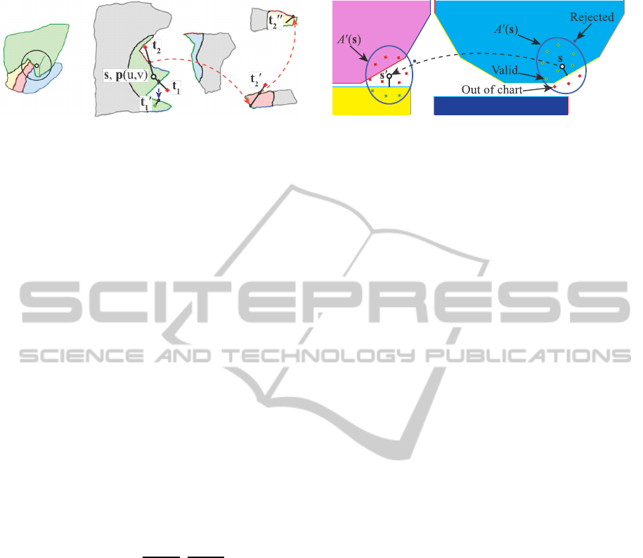
Figure 4: More examples of indexing samples. t

returns

to the same chart after a jump. t

parametric location is

located using two jumps. In the right part, chart adjacencies

are colored across the borders.

checking their respective chart identiﬁers ID(u,v) and

ID(u

′

In the case where t lands outside the chart of p,

we utilize the parametric adjacency data stored in our

buffers to ﬁnd its true location. Initially, we march

along the direction

−→

st in pixel-sized increments to lo-

cate the ﬁrst pixel with the chart ID as p (boundary

point b). The adjacency buffer for a border pixel b of

a chart contains the ID of the adjacent chart and the

parametric location b

′

of the corresponding point on

it. For samples across seams of the same chart, the

ID of the adjacent buffer is identical to that of p, but

the parametric location b

′

points safely to the corre-

sponding location on the same chart (see Figure 4-t

The adjacency buffer contains also the relative chart

edge rotation θ(b → b

′

) between b and b

′

. Finally, a

non-uniform scale factor s(b → b

′

) can be calculated,

corresponding to the relative scale of the two charts

in parametric space at their border locations b and b

′

(this scale factor may vary across a chart):

s(b → b

′

) =



′

)

(b)

′

)

(b)



. (2)

Therefore, we can adjust the location of t according to

the following parametric space transformation to ob-

tain the relocated sampling position t

′

on the adjacent

chart:

′

= b

′

+ R

θ(b→b

′

)

s(b→b

′

)

(t− b), (3)

where R

θ(b→b

′

)

is the rotation matrix of angle θ(b →

′

) and S

s(b→b

′

)

is the non-uniform scale matrix of

factor s(b → b

′

). In case t

′

lands outside the expected

chart, the same search is performed similarly in the

−→

′

direction (see Figure 4-t

). The sample reloca-

tion procedure is shown in Figure 3. Note that the full

non-rigid transformation of t corresponds to the adap-

tation of the initial sampling ellipse to the new charts.

Therefore, if no severe stretching is present, S(p) is

properly covered.

A useful side-effect of the parametric-space com-

putation is that feature estimation can take into ac-

Figure 5: Monte Carlo Sampling in current and adjacent

charts described in Section 4.1.

count displacement and normal mapping. In the spe-

cial case of displacement mapping, our method could

be easily adopted in order to handle the changes in

the geometry that could break the neighborhood esti-

mation heuristic. Points lying within the initial Eu-

clidean neighborhood that stretch out of it due to

the displacement are automatically handled by mea-

suring the Euclidean distance from p. The problem

arises when point with initial location outside the Eu-

clidean neighborhood of p fall within r

max

after dis-

placement. By scaling σ

and σ

with the maximum

expected displacement distortion, which is usually a

user deﬁned parameter, the method successfully han-

dles these points as well.

Finally, we need to clarify that if our method fo-

cused only on single chart parameterizations such as

Geometry images (Gu et al., 2002) we could avoid

highly irregular transitions and in this way reduce the

complexity of our operations. On the other hand,

multi-chart parameterizations offer an added ﬂexibil-

ity that can be used to reduce distortion, particularly

for shapes with long extremities, high genus, or dis-

connected components (Sander et al., 2003) (see Fig-

ure 13).

4 ESTIMATION OF INTEGRAL

FEATURES

Central to many geometric feature computations is

the estimation of surface and volume integrals in the

neighborhood of p. Integral invariant features for in-

stance, are often used in the formulation of local de-

scriptors (Huang et al., 2006), or provide the means

to estimate differential invariants such as the mean

curvature H (see (Connolly, 1986) and (Manay et al.,

2004)).

We estimate integrals in a neighborhood S(p)) us-

ing Monte Carlo integration in parametric space and

in Section 5 we use this approach to compute a va-

riety of integral and differential features interactively

for arbitrary feature scales.

AParametricSpaceApproachtotheComputationofMulti-scaleGeometricFeatures

4.1 Monte Carlo Integration

In parametric space, the generated data buffers hold

not only the vertex information but also all inter-

nal polygon samples, generated by the GPU through

linear interpolation during rasterization. Utilizing

Monte Carlo integration with a uniform distribution

in the parametric domain, any integral I(p) of a func-

tion g(p) over S(p) can be approximated by:

hIi(p) =

′

(s)

∑

i=1

g(P(t

)), (4)

where A

′

(s) is the portion of the elliptical sampling

area A(s) centered at parameter pair s corresponding

to the central point p = P(s) after rejection sampling

with the criterion of neighborhood S(p) (e.g. Eu-

clidean distance of P(t) to p) and N is the number of

valid samples. While performing a similar sampling

on the geometry itself would require area-weighted

probabilities, the parametric-space values can be sam-

pled uniformly, assuming of course a low-distortion

parameterization.

Random samples are generated uniformly using a

stratiﬁcation scheme. Uniform samples in the cells of

a planar grid are transformed to disk samples using

the concentric mapping of (Shirley and Chiu, 1997).

The disk samples are anisotropically scaled along the

u and v axes to form the elliptical region A(s), accord-

ing to the distortion factors discussed in Section 3.3.

The same samples are used at each pixel, randomly

rotating them to avoid statistical noise.

The elliptical region A(s) is an approximation that

favors fast computations. A more reﬁned but rather

more computationally expensive approach would be

to pre-compute the maximal distortion for discretized

polar coordinates at each pixel and subsequently

anisotropically scale each random sample according

to the closest distortion term from its conversion to

polar coordinates. Nevertheless, as demonstrated in

the experiments, the elliptical approximation proved

to be both robust and efﬁcient, even for large neigbor-

hoods.

Given a point p and its location in parametric

space s, initially we perform computations only for

the samples that lie on the same chart as p (Figure 5

- right). At the same time, for all parametric-space

samples that fall outside the chart, we mark the ID of

the chart they land on. Subsequently, we compute for

each marked chart the transformed parametric posi-

tion s

′

of the central parametric pair s and repeat the

sampling procedure on the new location, using the

entire sampling pattern (Figure 5 - left). Only sam-

ples falling within the new chart are accounted for and

contribute to the ﬁnal integral. The marking of charts

and the central point transformation is done according

to the procedure described in Section 3.4.

The sampling scheme described above is generic

and could be implemented for an arbitrary number of

jumps, excluding each time the already visited charts.

In our experiments we noticed that, no more than

one jump per sample point was typically required,

even for large-scale local feature neighborhoods. Of

course, this also depends on the size of the charts pro-

duced by the parameterization. For example, in Fig-

ure 2, where the bunny model is shown in two dif-

ferent parameterizations, for the left one we reported

the ﬁrst missing sample using a support area of 10%

the object’s diagonal. Conversely, for the one on the

right we did not report any missing samples even for

neighborhoods larger than 16% the object’s diagonal.

4.2 Adaptive Sampling

Since g(x) is a function of the surface geometry,

smooth areas of the objects, i.e. areas with smaller

variance of the evaluated function g(x), give satis-

factory results even when dropping the sampling rate

signiﬁcantly. This fact is an opportunity for a speed-

up, given that computation time is proportional to

the number of samples drawn, so we exploit adaptive

sampling to this end.

Typically, adaptive sampling methods continue to

draw random samples, until the variance of the com-

puted quantity falls below a certain threshold. In our

method however, we perform a simpliﬁed, two-step

adaptive sampling, instead of waiting for the variance

to converge: We ﬁrst compute the integral with N/2

samples and measure the variance. For those points p

for which the variance of g(x) is greater than a prede-

termined threshold, we use an additional set of N/2

random samples. Using a ﬁxed, two-stage adaptive

sampling creates exactly two different GPU execu-

tion loads, generally coherent across the output buffer,

thus maximizing shader core utilization and perfor-

mance.

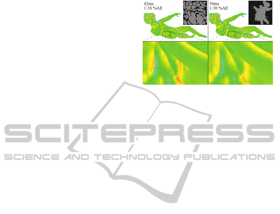
Our experiments show that as the number of sam-

ples increases, the difference of % Absolute Error (%

AE) between the full and adaptive sampling declines,

while at the same time the performance savings in-

crease. (see Table 1 and Figure 6).

5 PERFORMANCE AND

QUALITY EVALUATION

In this section we present a number of local geo-

metric feature operators using our method and pro-

vide a qualitative comparison against respective ref-

GRAPP2015-InternationalConferenceonComputerGraphicsTheoryandApplications

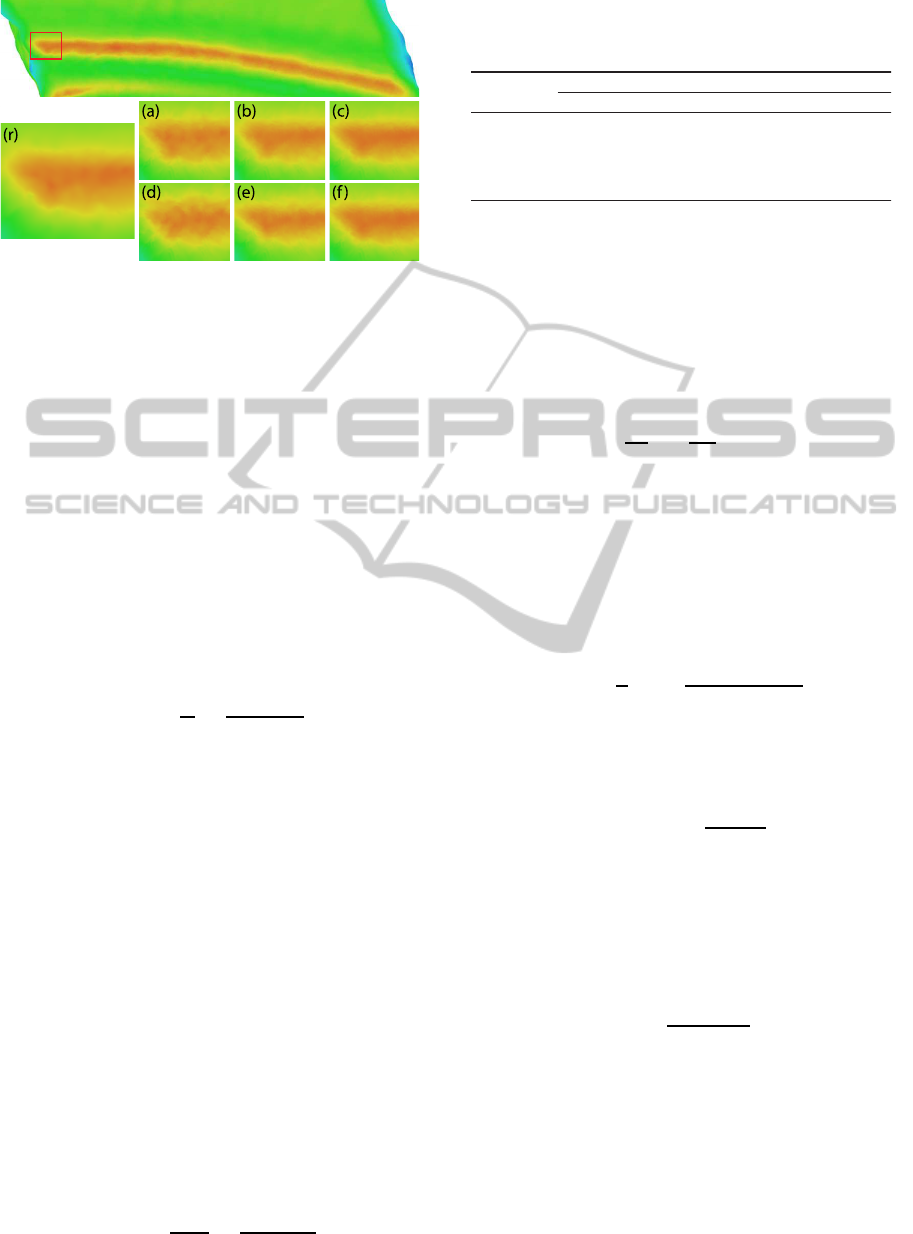
Figure 6: Comparison of mean curvature for Full and Adap-

tive Sampling. (r) Reference (a), (b), (c) Full Sampling us-

ing 64, 100 and 256 samples in respect. (d), (e), (f) Adaptive

Sampling using 32/64, 64/128 and 128/256 samples.

erence CPU algorithms that operate directly on the

polygonal geometry using the Halfedge data-structure

(HE) (Campagna et al., 1998).

5.1 Implemented Local Features

Local Bending Energy (LBE). (Huang et al., 2006)

in order to classify a surface as fractured or intact in

their fragment reassembly framework deﬁne the LBE

term e

(p) for the k nearest vertices to a surface lo-

cation p. Similarly, given an Euclidean neighborhood

∈ S(p,r) : kq

− pk ≤ r with corresponding normal

vectors n

, LBE e

(p) can be deﬁned as:

(p) =

∑

i=1

kn− n

kp− q

, (5)

where n is the normal at the central point p and

N is the number o samples taken in the S(p,r)

neighborhood.

Sphere Volume. (McGuire et al., 2011) presented

a stochastic solid angle computation for the approx-

imation ambient occlusion in the hemisphere above

a point p. Inspired by this idea, we extend it to a

full sphere and compute a fast approximation of the

unoccupied volume of a sphere of radius r centered

at p. Assuming a smoothly varying tangential eleva-

tion around p, the vector q

− p from the central point

to any sample q

within the Euclidean neighborhood

S(p,r) approximates the horizon in this direction with

respect to the normal vector n at p at a distance scale

equal to kq

− pk. Taking a uniform rotational and ra-

dial distribution of samples (direction and scale) q

S(p,r), we can approximate the open volume V

(p)

above p by:

(p) =

4πr

∑

i=1

− p)n

− pk

. (6)

Table 1: Computation Time and % Absolute Error for Full

and Adaptive Sampling over the same metric. Error in com-

parison to reference CPU implementation.

Samples

Full Adaptive

Time

% AE

Time

% AE

64 17.57ms 1.172 15.94ms 1.331

100

22.17ms

1.035 19.54ms 1.110

256 50.54ms 1.005 41.44ms 1.007

400 74.21ms 0.789 61.75ms 0.824

The sphere volume integral invariant, i.e. the part of

the sphere volume of radius r ”inside” the surface at

p (Pottmann et al., 2009) is the complement of the

above integral quantity.

Mean Curvature (MC). (Hulin and Troyanov, 2003)

derive the relation of MC to the sphere volume inte-

gral invariant as:

(p) =

2π

−

πH

+ O(r

), (7)

from which we can directly compute MC H at p for a

given radius r.

Shape Index (SI). Introduced by (Koenderink and

van Doorn, 1992), SI is a local descriptor that com-

bines the principal curvatures (PC) in order to classify

the locale shape of the surface. SI is a normalized de-

scriptor and for a given surface point p is deﬁned as:

S(p) =

arctan

(p) + K

(p)

(p) − K

(p)

, (8)

where K

(p), K

(p) are the principal curvatures at p.

In order to calculate the K

and K

, we rely on

their relation to mean curvature H and Gaussian cur-

vature (GC) K:

1,2

= H ±

− K. (9)

The computation of H was discussed earlier. For the

GC we rely on the work of (Bertrand et al., 1848)

that relates K with the perimeter and surface area of

a geodesic disk on a surface. In particular, we utilize

the formula that uses the geodesic area GA of distance

K = 12

πr

− GA

πr

. (10)

The only unknownparameter now is the geodesic area

at a given distance r. In the case of the geo-

metric evaluation, we sum the Voronoi area of each

vertex within a neighborhood of geodesic distance r.

For the parametric-space computation of GA

, we ﬁrst

draw a number of samples N

tot

in the Euclidean neigh-

borhood of p (see Section 4.1). Then, for each sam-

ple q

at parametric location t

, the geodesic distance

to p is approximated by a sum of chords at P(s

AParametricSpaceApproachtotheComputationofMulti-scaleGeometricFeatures

13600ms 129ms

%AE: 1.17

Arc

900K Triangles

250x170x136mm

5mm Radius

Armadillo

345K Triangles

126x115x152mm

2mm Radius

2130ms 134ms

%AE: 1.88

Parametric SpaceReference

9410ms 47ms

%AE: 0.81

Arc

900K Triangles

250x170x136mm

6mm Radius

XYZ RGB Dragon

200K Triangles

200x132x90mm

3mm Radius

397ms

52ms

%AE: 1.89

624ms 28ms

%AE: 1.18

Embrasure

200K Triangles

340x334x330mm

10mm Radius

Armadillo

345K Triangles

126x115x152mm

3mm Radius

1420ms

55ms

%AE: 1.41

Parametric SpaceReference

113ms 21ms

%AE: 0.31

Embrasure

200K Triangles

340x334x330mm

3mm Radius

Lucy

200K Triangles

345x134x400mm

6mm Radius

360ms 57ms

%AE: 1.08

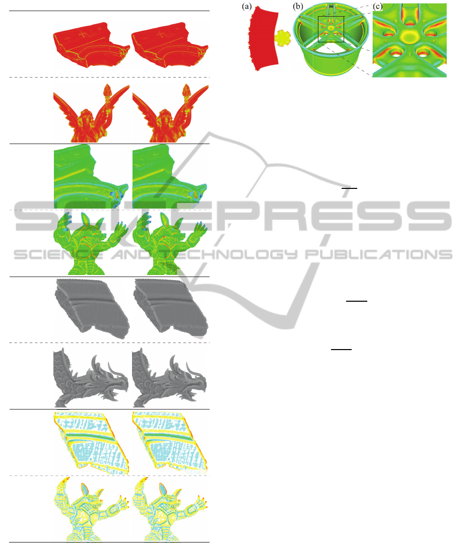
Localized Bending EnergyMean CurvatureShape Index Normalized Sphere Volume

Figure 7: Comparative visualization, timings and % Ab-

solute Error for the implemented geometric features (Sec-

tion 5.1).

i.e. at the intermediate parametric space coordinates

= t

+ j(s − t

)/N

steps

, where s are the uv coordi-

nates of p and N

steps

is the number of chords. Depend-

ing on the local distortion of the parameterization,

Figure 8: Genus 20 Rim model. a) Parametric space charts.

b) Mean Curvature colorized for the same neighborhood

computed in 58ms. c) Zoom to detail.

P(s

) may not reside exactly on the same plane. Ac-

cording to the computed geodesic distance between q

and p, a ﬁnal set of N

samples is retained, N

≤ N

tot

and GA

is estimated by:

tot

, (11)

where EA

is the Euclidean area.

Euclidean area can be approximated in the follow-

ing way. Let P

tot

be the total number of pixels in

the elliptical region. Given the ratio of the samples

that satisfy the Euclidean criterion to the total sam-

ples N

A(s)

tot

, and A

the mean area represented by

each sample in A(s), we approximate EA

as:

= P

tot

A(s)

tot

, (12)

is given by the formula:

A(s)

∑

i=1

, (13)

where A

is the product of the distortion factors

(u,v), l

(u,v).

5.2 Results and Discussion

We have tested our generic parametric-space feature

estimation method using a large variety of objects,

ranging from simple geometric shapes to complex and

detailed 3D scanned models. Indicative results can be

seen in Figure 7 and Figure 8, where we report an av-

erage of 49× acceleration and 1.245% Absolute Error

(AE) relative to the reference CPU method described

below. Please note that in such comparisons, report-

ing maximum error is not indicative of the method’s

performance, since a slight mismatch in the represen-

tation at a single point due to parameterization can

cause an isolated but inconsequential measurement

difference. Timings of our method do not include the

parameterization and the charts boundary edge detec-

tion. Similarly, timings of the reference method do

not include the Half-Edge (HE) data structure gen-

eration. It is importnat to mention here that while

geometric algorithms for computing features operate

GRAPP2015-InternationalConferenceonComputerGraphicsTheoryandApplications

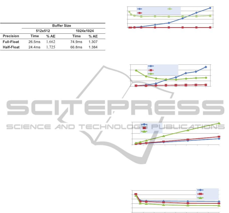
Table 2: Average Computation time and % Absolute Error

over a set of models for the same metric over different res-

olutions and buffer precision. Error in comparison to the

reference CPU implementation.

on discretized values at a vertex or triangle level, the

parametric space calculations can exploit interpolated

values at arbitrary surface locations. Therefore, the

measurement deviations that are reported here as er-

rors, mostly stem from the different approximation

and sampling of the underlying surface. Timings for

the GPU parametric implementation are shown for an

NVIDIA GTX 670 GPU. We use 1024x1024 ﬂoating

point texture buffers, while metrics are computed over

a 512x512 buffer with 256 samples per pixel unless

stated otherwise. The reference geometric algorithm

results are shown for a Corei7-3820 system (4 cores

@ 3.60GHz, 8 threads) with 16GB of RAM and our

implementation uses the OpenMP API and takes ad-

vantage of the current generation multi-core CPU’s.

The efﬁciency of our method is attributed to the

shift of the computations from a topology-detail-

dependent representation to two dimensions with

application-controlled (sampling) quality settings,

which enables very good scaling for multi-core and

many-core architectures. The proposed implemen-

tation is tailored for (but not limited to) commodity

GPUs.

Geometric Detail. In Figure 9 we present compar-

ative results computed over a ﬁxed neighborhood

size (4% of object’s diagonal) for a single model

(Embrasure) decimated at different geometric detail

levels. For small resolutions (25K, 50K triangles) we

observe similar computation times between geomet-

ric and parametric space approaches, while the %AE

is high in comparison to higher detail versions of

the mesh. This is expected as the parametric method

uses the position samples as interpolated by the GPU

resulting in smoother and therefore slightly different

results than the CPU method. For larger resolutions,

we report an acceleration of 3× for the 100K model

to 137× for the 1000K model, with a steady AE.

Finally, for the original scanned object resolution of

1200K, we report a 181× faster computation with

a slight increase in the %AE. This is also expected

and attributed to the relative small buffer size for

the dense geometric detail. However, this can be

trivially addressed by increasing the geometry buffer

resolution to 2048x2048.

200K 400K 600K 800K 1M 1.2M

Time in Seconds

Number of Triangles

Object Space

Parametric Space

0.4

0.8

1.2

1.6

% Absolute Error

%AE

Scalability over Geometric Density

Figure 9: Computations using the same metric and neigh-

borhood size (Left axis). Green line shows the %AE of the

parametric method (Right axis).

15x

23x

30x

2% 4% 6% 8% 10% 12% 14% 16%

Computation Time

Size of Neighborhood (% object diagonal)

Scalability over Neighborhood Size

Object Space

Parametric Space

0.00

0.80

1.60

2.40

3.20

% Absolute Error

%AE

Figure 10: Computations using the same metric and geo-

metric complexity (Left axis). Green line shows the %AE

of the parametric method (Right axis).

200

150

100

50 100 150 200 250 300 350 400

Time in Milliseconds

Number of Samples

Performance Control

512/512

1024/512

1024/1024

Figure 11: Average performance over several models us-

ing different number of samples, buffers size and size of

texture over which computations are performed. Legends

show Buffers Texture/Computations Texture Size in square

format.

1024/512

512/512

0.5

1.0

1.5

2.0

2.5

3.0

0 50 100 150 200

250

300

350

400

% Absolute Error

Number of Samples

Quality Control

1024/1024

Figure 12: Average quality over several models using differ-

ent number of samples, buffers size and size of texture over

which computations are performed. Legends show Buffers

Texture/Computations Texture Size in square format.

Neighborhood Size. In the measurements of Fig-

ure 10 we shift the focus from the geometric detail to

neighborhood size. Results are for the same model

(Embrasure) and metric (mean curvature) at 600K

resolution. We notice that for small neighborhoods

the %AE is higher. This deviation between the

parametric and geometric domain results are due

to the inadequate discrete representation of the

neighborhood in the geometric solution. While in the

parametric domain due to the interpolation of values

we mentioned earlier, an increasing neighborhood

AParametricSpaceApproachtotheComputationofMulti-scaleGeometricFeatures

size is directly reﬂected in a wider selection of

samples, the geometric neighborhood expands in

n-ring discrete steps, which is actually a deﬁciency.

For very large neighborhoods we notice also an

increase to the %AE, this time, due to the one jump

per sample approach of our implementation (see

end of Section 4.1), which starts missing samples.

Performance-wise, the parametric space method

scales very well and proves unaffected by the 8×

growth of neighborhood size. More speciﬁcally, the

computation time for the parametric domain feature

estimator grows by 2.25 times in contrast to the

26.45× factor reported by the geometric approach.

Performance and Quality Control. The number

of samples per pixel, buffer size and size of the

texture over which computations are performed, are

parameters that control the quality/performance of

our method. As we can see in Figure 11, increasing

the number of samples reduces the %AE and has

linear impact on the computation time, regardless

of the buffer resolution. The same effect have the

buffer size and the size of the texture over which

computations are performed (see Figure 12). Using

these parameters, performance and quality can be

controlled depending on the application requirements.

Memory Usage - Texture Size and Precision.

Four RGBA textures are used (see Section 3.3).

All the presented results so far were performed

using half-ﬂoat precision textures. In order to

evaluate the performance/quality impact of full-ﬂoat-

precision textures (FF), which double the memory

requirements, we performed experiments using both

resolutions (Table 2). FF buffers present an 8%

and 11% performance degradation on 512x512 and

1024x1024 buffers respectively, while the corre-

sponding improvement in AE is 4% and 6%. We can

conclude that the minor quality improvement does

not justify the performance drop and the doubled

memory requirements.

UV Parameterization. In order to evaluate how our

method is affected by the underlying parameterization

in terms of speed and quality, we performed several

tests. When operating on maps coming from global

surface parameterization (single chart) techniques, we

notice faster times, and increased error rates (see Fig-

ure 13) compared to multi-chart parameterizations

opting for minimal stretching. Single charts, mini-

mize branching operations but at the same time result

in greater distortion and less uniform sampling lead-

ing thus in loss of representation and measurement

accuracy.

Figure 13: Mean Curvature (Colorized) computed using

different parameterizations. Multiple charts result in in-

creased computation times, but smaller error, due to the

smaller distortion of the generated charts.

6 LIMITATIONS

Due to the fact that parameterization of the objects

surface is required, the method is limited to mesh ge-

ometries and it cannot be directly applied on point-

clouds.

7 CONCLUSION AND FUTURE

WORK

We presented a novel generic parametric-space ap-

proach for the computation of geometric features in

multiple scales. Decoupling of computational com-

plexity from the underlying geometry and the scale of

the features, leads to a fast, real-time method, suitable

for deformable/animated objects.

As future work we intent to evaluate the per-

formance of demanding applications, such as object

matching, object retrieval etc. using the parametric-

space computations.

ACKNOWLEDGEMENTS

This work was supported by EC FP7 STREP Project

PRESIOUS, grant no. 600533. Armadillo, Lucy,

Bunny and XYZ RGB Dragon models are from

Stanford 3D Scanning Repository. Angel model is

from the Large Geometric Models Archive of Geor-

gia Institute of Technology. Rim model is from

http://www.turbosquid.com. All other models used

are from the PRESIOUS project data collection.

GRAPP2015-InternationalConferenceonComputerGraphicsTheoryandApplications

REFERENCES

Bertrand, J., Diquet, C., and Puiseux, V. (1848).

D´emonstration d’un th´eor`eme de Gauss. Journal de

Math´ematiques, 13:80–90.

Campagna, S., Kobbelt, L., and Seidel, H.-P. (1998). Di-

rected edges—a scalable representation for tri-

angle meshes. J. Graph. Tools, 3(4):1–11.

Connolly, M. L. (1986). Measurement of protein surface

shape by solid angles. J. Mol. Graph., 4(1):3–6.

De Floriani, L. and Hui, A. (2005). Data structures for sim-

plicial complexes: An analysis and a comparison. In

Proc. of the Third Eurographics Symp. on Geometry

Processing, SGP ’05. Eurographics Association.

Floater, M. and Hormann, K. (2005). Surface parameteriza-

tion: a tutorial and survey. In Advances in Multireso-

lution for Geometric Modelling, Mathematics and Vi-

sualization, pages 157–186. Springer.

Grifﬁn, W., Wang, Y., Berrios, D., and Olano, M. (2011).

GPU curvature estimation on deformable meshes. In

Symp. on Interactive 3D Graphics and Games, I3D

’11, pages 159–166. ACM.

Gu, X., Gortler, S. J., and Hoppe, H. (2002). Geometry

images. In Proc. of the 29th Annual Conference on

Computer Graphics and Interactive Techniques, SIG-

GRAPH ’02, pages 355–361. ACM.

Hormann, K., Polthier, K., and Sheffer, A. (2008). Mesh

parameterization: Theory and practice. In ACM SIG-

GRAPH ASIA 2008 Courses, SIGGRAPH Asia ’08,

pages 12:1–12:87. ACM.

Hua, J., Lai, Z., Dong, M., Gu, X., and Qin, H. (2008).

Geodesic distance-weighted shape vector image diffu-

sion. IEEE Trans. Vis. Comput. Graph., 14(6):1643–

1650.

Huang, Q.-X., Fl¨ory, S., Gelfand, N., Hofer, M., and

Pottmann, H. (2006). Reassembling fractured ob-

jects by geometric matching. ACM Trans. Graph.,

25(3):569–578.

Hulin, D. and Troyanov, M. (2003). Mean curvature and

asymptotic volume of small balls. The American

Mathematical Monthly, 110(10):947–950.

Kim, Y., Yu, J., Yu, X., and Lee, S. (2008). Line-art il-

lustration of dynamic and specular surfaces. In ACM

SIGGRAPH Asia 2008 Papers, SIGGRAPH Asia ’08,

pages 156:1–156:10. ACM.

Koenderink, J. J. and van Doorn, A. J. (1992). Surface

shape and curvature scales. Image Vision Comput.,

10(8):557–565.

Manay, S., Hong, B.-W., Yezzi, A., and Soatto, S. (2004).

Integral invariant signatures. In Computer Vision -

ECCV 2004, volume 3024 of Lecture Notes in Com-

puter Science, pages 87–99. Springer.

McGuire, M., Osman, B., Bukowski, M., and Hennessy, P.

(2011). The alchemy screen-space ambient obscu-

rance algorithm. In Proc. of the ACM SIGGRAPH

Symp. on High Performance Graphics, HPG ’11,

pages 25–32. ACM.

Mellado, N., Barla, P., Guennebaud, G., Reuter, P., and

Duquesne, G. (2013). Screen-space curvature for

production-quality rendering and compositing. In

ACM SIGGRAPH 2013 Talks, SIGGRAPH ’13, pages

42:1–42:1. ACM.

Meyer, M., Desbrun, M., Schrder, P., and Barr, A. (2003).

Discrete differential-geometry operators for triangu-

lated 2-manifolds. In Visualization and Mathemat-

ics III, Mathematics and Visualization, pages 35–57.

Springer.

Museth, K. (2013). Vdb: High-resolution sparse vol-

umes with dynamic topology. ACM Trans. Graph.,

32(3):27:1–27:22.

Novatnack, J. and Nishino, K. (2007). Scale-dependent 3D

geometric features. In Computer Vision, 2007. ICCV

2007. IEEE 11th International Conference on, pages

1–8. IEEE.

Pottmann, H., Wallner, J., Huang, Q.-X., and Yang, Y.-L.

(2009). Integral invariants for robust geometry pro-

cessing. Comput. Aided Geom. Des., 26(1):37–60.

Pottmann, H., Wallner, J., Yang, Y.-L., Lai, Y.-K., and Hu,

S.-M. (2007). Principal curvatures from the integral

invariant viewpoint. Computer Aided Geometric De-

sign, 24(8):428–442.

Rusinkiewicz, S. (2004). Estimating curvatures and their

derivatives on triangle meshes. In Proceedings of

the 3D Data Processing, Visualization, and Trans-

mission, 2Nd International Symposium, 3DPVT ’04,

pages 486–493. IEEE Computer Society.

Sander, P. V., Snyder, J., Gortler, S. J., and Hoppe, H.

(2001). Texture mapping progressive meshes. In Proc.

of the 28th Annual Conference on Computer Graphics

and Interactive Techniques, SIGGRAPH ’01, pages

409–416. ACM.

Sander, P. V., Wood, Z. J., Gortler, S. J., Snyder, J., and

Hoppe, H. (2003). Multi-chart geometry images.

In Proc. of the 2003 Eurographics/ACM SIGGRAPH

Symp. on Geometry Processing, SGP ’03, pages 146–

155. Eurographics Association.

Sheffer, A., Praun, E., and Rose, K. (2006). Mesh pa-

rameterization methods and their applications. Found.

Trends. Comput. Graph. Vis., 2(2):105–171.

Shirley, P. and Chiu, K. (1997). A low distortion map be-

tween disk and square. J. Graph. Tools, 2(3):45–52.

Taubin, G. (1995). Estimating the tensor of curvature of a

surface from a polyhedral approximation. In Proceed-

ings of the Fifth International Conference on Com-

puter Vision, ICCV ’95, pages 902–. IEEE Computer

Society.

Yang, Y.-L., Lai, Y.-K., Hu, S.-M., and Pottmann, H.

(2006). Robust principal curvatures on multiple

scales. In Symp. on Geometry Processing, pages 223–

226.

Yoshizawa, S., Belyaev, A., and Seidel, H.-P. (2004). A

fast and simple stretch-minimizing mesh parameteri-

zation. In Proc. of the Shape Modeling International

2004, SMI ’04, pages 200–208. IEEE Computer Soci-

ety.

Zhou, K., Synder, J., Guo, B., and Shum, H.-Y. (2004).

Iso-charts: Stretch-driven mesh parameterization us-

ing spectral analysis. In Proc. of the 2004 Eurograph-

ics/ACM SIGGRAPH Symp. on Geometry Processing,

SGP ’04, pages 45–54. ACM.

AParametricSpaceApproachtotheComputationofMulti-scaleGeometricFeatures