Crater Detection using CGC

A New Circle Detection Method

Vinciane Lacroix

and Sabine Vanhuysse

CISS Department, Royal Military Academy, Brussels, Belgium

IGEAT, Universit´e Libre de Bruxelles, Brussels, Belgium

Keywords:

Circle Detection, Crater Detection, Constrained Gradient, Feature Extraction.

Abstract:

”Constrained Gradient for Circle” (CGC) is a new circle detection algorithm based on the gradient of the

intensity image. The method relies on two conditions. The “gradient angle compatibility condition” constrains

the gradient of a given percentage of the pixels belonging to some digital circles having a radius in the range of

radii to detect to point towards the centre of the circle or in the opposite direction. The “curvature compatibility

condition” constrains the variation of the gradient angle of the same pixels in a range depending on the radius

of the circle. These two conditions are sufﬁcient to detect the core of circular shapes. The best-ﬁtting circle

is then identiﬁed. The method is applied to artiﬁcial and reference images and compared to state-of-the-art

methods. It is also applied to water-ﬁlled crater detection in Cambodia: these craters that might indicate

the presence of Unexploded Ordnance (UXO) dating from the US bombing produce dark circles on satellite

panchromatic images.

1 INTRODUCTION

The presence of Unexploded Ordnance (UXO) result-

ing from the US bombing during the late 1960s and

1970s is still preventing the use of the land in Cam-

bodia. When dropped, the bombs produced craters

that may still exist today. Many of them are ﬁlled

with water so that they appear as circular objects on

panchromatic satellite images. The purpose of this

study is to extract those craters as they might indicate

the presence of UXOs. Similar work was made by

Hatﬁeld Consultants (Hatﬁeld-Consultants, 2014) for

Laos. The authors used historic Corona satellite im-

ages; they computed differences between the original

image and its smoothed version, and used these dif-

ferences in an unsupervised K-means fuzzy classiﬁer.

One class contained the impacted areas which were

then identiﬁed based on geometrical characteristics.

The geometry (i.e. the fact that craters are almost cir-

cles) is being used at the end of the process whereas

our approach is rather to start with geometry, i.e. dark

circle detection.

Circle detection has been a challenge since the

early days of Pattern Recognition and is still arous-

ing interest as recent publications show ((Chung et al.,

2012), (Akinlar and Topal, 2013), (Marco et al.,

2014)). Exhaustive review of circle detection meth-

ods can be found in the introduction of these arti-

cles. “Circle” may designate the border of a “sphere”,

“disc” or “ring”, or, a very thin ring, as shown on Fig-

ure 1. In this publication, we are interested in “disc”

detection, although the proposed method can be used

as such for sphere detection and for detecting inner

ring circumference. The method may be adapted for

the detection of the other types of circles but such an

adaptation is not described here.

(a) (b) (c) (d)

Figure 1: (a) Sphere; (b) disc; (c) ring; (d) thin ring.

ough transforms and their randomised ver-

sions are very popular (see for example (Xu et al.,

1990),(Yip et al., 1992)) but are still very time con-

suming as they rely only on the hypothesis of three

edgels belonging to a circle and they may require

complex structures for storing the votes. Some com-

putational time may however be saved using the gra-

dient orientation to constrain edgels belonging to the

same circle (see for example (Atherton and Kerbyson,

1999)) or using a LUT method ((Chung et al., 2009)).

320

Lacroix V. and Vanhuysse S..

Crater Detection using CGC - A New Circle Detection Method.

DOI: 10.5220/0005222503200327

In Proceedings of the International Conference on Pattern Recognition Applications and Methods (ICPRAM-2015), pages 320-327

ISBN: 978-989-758-076-5

 2015 SCITEPRESS (Science and Technology Publications, Lda.)

Most existing approaches use the fact that some

basic elements (pixels, edgels, or connected seg-

ments) are part of the circumference and combine

some of them to generate a centre-radius pair hypoth-

esis. To our knowledge, none of them uses a “blind”

centre-radius hypothesis as detecting circles of vari-

ous radii at each pixel seems time-consuming.

However, performing a ﬁrst test on the gradient

angle on a few pre-deﬁned digital circles of radius

spanning the radius range to detect allows to isolate

the core of shapes (circle, ellipses, squares, etc.) of

the corresponding size. This test requires the gradi-

ent angle of pixels located on the digital circles to be

similar to the angle of the line joining the pixel to

the circle centre. The second test consists in check-

ing if the gradient angle variation of pixels located

on the same circle are compatible with the one asso-

ciated with the considered circle. The second test en-

ables to keep circular shapes only. A counter is set at

each pixel considered as a potential centre and is in-

cremented if both tests are positive for the considered

digital circle. The percentage of compatible pixels is

stored and if the counter represents a signiﬁcant part

of the digital circle, the centre is considered as a po-

tential candidate.

A second phase is however necessary to identify

the best centre/radius pair among the candidates. In

order to ease the second phase, in this publication, we

assume that the circles present in the image do not

overlap, and thus, if there is a circle at some pixel,

it is unique. This assumption is valid for the crater

detection application we are concerned with but might

not be true for other applications.

As the method is based on constrains on the gra-

dient, it is called ”CGC” meaning ”Constrained Gra-

dient for Circle”.

This paper is organized as follows. Section 2

presents the ﬁrst phase aiming at extracting centres

candidates. In that section, the gradient angle and the

curvature compatibility conditions are presented. The

algorithm is then described and applied to an artiﬁcial

image. In Section 3, a second phase aimed at extract-

ing the best centre-candidate and the adequate circle

is proposed. In Section 4 the results of the full pro-

cess applied to three different images are presented

and compared to the ones of state-of-the-art methods.

Discussion and conclusions are provided in Section 5.

2 EXTRACTING CENTRES

CANDIDATES

In natural images or in scanned graphics, pure step

edges are not very probable; edges are rather span-

Intensity

Gradient Norm

Intensity

Gradient Norm

(c)

(d)

(b)

(a)

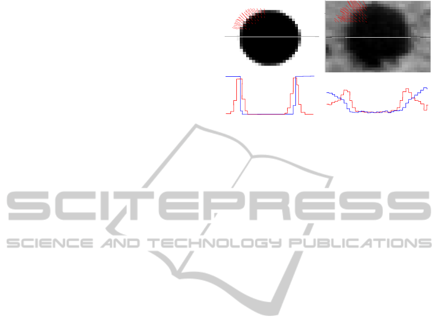
Figure 2: (a) Scanned graphic and (b) natural image with

some scaled gradient vectors overlayed and in (c-d) their

respective Intensity (in blue) and gradient norm proﬁles (in

red) at the centre line.

ning over a few pixels, which makes hills of gradient

norm even broader; in this study we use the Gaussian

gradient (Canny, 1986) with σ = 1. In the vicinity of

the border of a circle, the gradient orientation is near

the line passing through the centre, although the dis-

cretization process makes it dependent on the angle

and position (see Figure 2). Moreover, the variation

of the gradient angle in the direction perpendicular to

the gradient depends on the distance of the pixel to

the centre. These properties are exploited in the ﬁrst

phase of the process.

2.1 Compatibility Conditions

2.1.1 Gradient Angle

In order to have a circle of radius r at centre c, all

gradient vectors located on the digital version of the

circle should point either towards c (bright circle)

or in the opposite direction (dark circle); because of

the discretization process, they will not point exactly

along this direction, but the angle difference should

be small (see the examples of Figure 2).

Let angles be expressed in fraction of radian (i.e.

unit= radian/π) so that the angle range is [−1 1]. Let

p be a pixel located on a digital circle C of radius r at

centre c, let γ be the gradient angle at p, and let α be

the angle of the line joining p to c. If there exists a cir-

cle of radius r at c, the gradient angle compatibility

condition at c is deﬁned as: ∀p ∈ C,

Diff(α− γ) < ε

for dark circle

Diff(α− (1− γ)) < ε

for bright circle (1)

where Diff denotes angle difference.

This condition is necessary but not sufﬁcient: it is

also true for “centres” of other shapes such as circles

of radius r

′

close to r (depending on the edge proﬁle

CraterDetectionusingCGC-ANewCircleDetectionMethod

321

and on the extent of the ﬁlter in the gradient compu-

tation), for ellipses of axis close to r, and for shapes

ﬁtting in circles of similar radius values. Moreover,

depending on the tolerance on the angle difference ε

the condition in (1) will not only hold for the centre

of the shape but also for its neighbourhood.

2.1.2 Gradient Angle Variation

If p is located on a digital circle, the local variation of

the angle of the gradient is also constrained. Let s and

t the two points located at a distance δ in the direction

perpendicular to the gradient at p. Let κ be deﬁned

according to the Equation 2.

κ = Diff(γ

− γ

) (2)

where γ

and γ

denote the gradient angle at s and t.

κ is an approximation of the local curvature at p and

will abusively called “curvature” in the following. If

r is the radius of the circle, κ is such that

κ = 2∗ arcsin(δ/r) (3)

Some tolerance on the curvature should also be

allowed to deal with the discretization process. Thus

the curvature compatibility condition at c is de-

ﬁned as: ∀p ∈ C,

2∗ arcsin(δ/r) − ε

< κ

< 2∗ arcsin(δ/r) + ε

− ε

< κ

+ ε

(4)

where ε

designates the toleranceon the curvature and

the curvature at p.

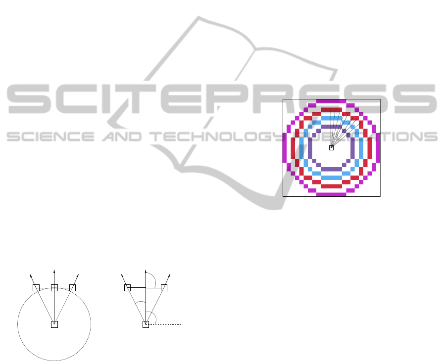
Figure 3 illustrates the two constraints for a pixel

p located at angle α on the circle C of radius r = 6.

κ/2

s t

c c

Figure 3: Constraint on gradient angle γ and on curvature κ

at p located on circle C of radius r; s and t are located at a

distance δ of p in the direction perpendicular to γ.

In the case of an imperfect or partial circle of ra-

dius r, only a fraction f of the gradient angles located

on C will satisfy condition (1) and (4). The number of

pixels n that should satisfy the angle and the curvature

compatibility condition, and b, the maximum number

of non-valid pixels are thus deﬁned by

n = f # C and b = (1− f) # C (5)

where # denotes the cardinality.

If the circles to detect have a radius between rmin

and rmax, thanks to the smooth variation of the gradi-

ent direction in the direction perpendicular to the bor-

der (see Figure 2), not all correspondingdigital circles

need to be tested for angle and curvature compatibil-

ity. In this publication we use all integer values of r

between rmin and rmax by step of two.

There exist several implementations of digital cir-

cles (Blinn, 1996). In this study, the pixels of the dig-

ital circle C of radius r are found by starting at pixel

p(i, j) = (0,r), incrementing i by one, computing j

using the circle equation, and computing the angle us-

ing arcsin until 0.25 (π/8)) is reached; the other pix-

els are found using the circle symmetries (see some

resulting circles in Figure 4). The chosen implemen-

tation — also known as Bresenham’s circle algorithm

— is the one that has the smallest number of pixels

while preserving the connectivity.

Figure 4: Digital circles used in this study for a radius range

from 5 to 12 and a few vectors joining the centre to the

pixels lying on the circle of radius r = 9 ; each digital circle

is displayed in a different color.

2.2 Phase One: Algorithm Description

2.2.1 Prerequisite

1. Compute Gaussian gradient G

, G

and norm N.

2. Compute Angle of gradient A, and curvatureK ac-

cording to Equation 2.

2.2.2 Centre Candidates

Let ε

, ε

, f and t be the tolerance on gradient angle,

the tolerance on curvature, the fraction of circle to de-

tect and the threshold value under which the norm of

gradient is considered as noise respectively.

1. Let C = {C

,..,C

,...C

} be the list of digital

circles located at the origin, corresponding to the

increasing radii r

,...r

,..r

with rmin = r

and

≤ rmax. For each C

, get the list of vectors p

joining the centre to each pixel located on the dig-

ital circle (i.e. using Bresenham’s algorithm) and

their angle a

; compute z

= # C

, b

and n

ac-

ICPRAM2015-InternationalConferenceonPatternRecognitionApplicationsandMethods

322

cording to Equation 5 and the ideal curva-

ture κ

according to Equation 3.

2. Initialize two rasters R andV for storing the radius

and the fraction of valid pixels.

3. Scan the image; for each pixel c, compute the

fraction of valid pixels lying on the digital circles

,..,C

,...C

} starting with the smallest circle

, as follows. For each vector p

of C

, get the

pixel q

= c + p

, lying on circle C

centred at c

and test three conditions:

• the minimum norm condition: N

> t;

• the angle difference compatibility condition ac-

cording to Equation 1, where α = a

(angle of

) and γ = A

(gradient angle at q

);

• the curvaturecompatibility condition according

to Equation 4 where κ is the curvature at q

and

= κ

If all conditions are satisﬁed, increment the

“good” counter at c (count separately dark and

bright circle according to the gradient angle at

), otherwise increment the “bad counter”. As

soon as the bad counter has reached b

, the next

circle C

i+1

is tested. Otherwise, test the full circle

, save r (radius) and v (fraction of valid pixel) in

R and V respectively. For convenience purpose, a

negative value in V indicates a dark circle. Store

c in a list of potential centre candidates.

2.2.3 Shapes’ Core

Get the connected components of all centre candi-

dates. In the case of non-overlapping circles, each

connected component will be the core of a circular

shape. For each connected components, compute c

the centre of gravity of the pixels with the lowest ra-

dius r (it should be a centre candidate, but if it is not,

consider the 8-neighbours of similar radius with the

highest counter). c

−r is a ﬁrst centre-radius approx-

imation of the shape.

2.3 Application

The parameters of the proposed method are:

• σ = 1 and δ = 2 for the prerequisite Gaussian gra-

dient and curvature computation,

• t = 10 for ignoring pixels with a too low gradient

norm,

• ε

, ε

, for setting the tolerance on gradient angle

and curvature; expressed in fraction of radian (i.e.

unit= radian/π), a reasonable range is [0.06 0.14].

For simplicity ε

= ε

• f, for the minimal fraction of circle to detect. A

reasonable range is [0.7 1];

The fraction of detected circle v at some potential cen-

tre depends on ε

/ε

: if the tolerance rises, the portion

of detected circle will stay equal or become larger.

The parameters f and ε

/ε

are thus not independent.

Experiments on geometric ﬁgures on a uniform

backgroundprovide some insight on the method (used

with rmin = 5 and rmax = 15) and enable to analyse

the effect of the parameters ε

, ε

, and f on the pro-

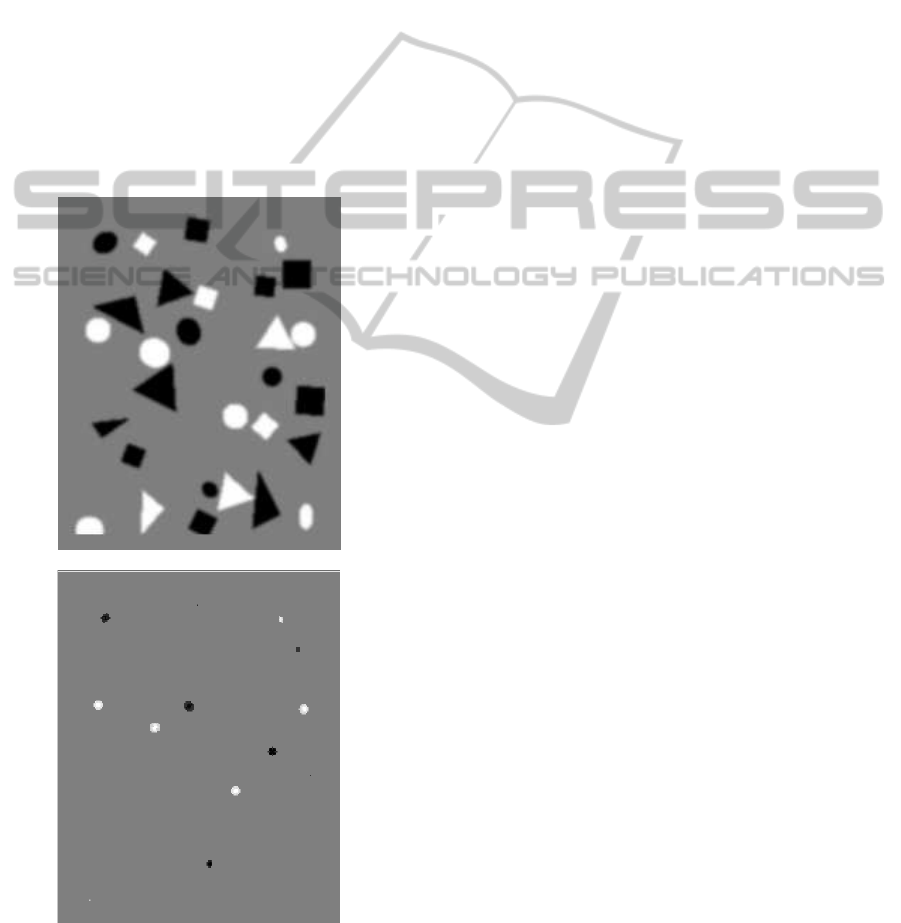
duction of candidates. The shapes are identiﬁed by

numbers on Figure 5 (top). The raster V displaying v,

the fraction of the smallest valid circle at each centre

candidate, has been analysed for values of ε = ε

= ε

ranging from 0.06 to 0.14, and f = 0.6. Although

0.6 is below the recommended value, it enables to

see when false alarms occur for low f values. An

example of such a raster is shown on Figure 5 (bot-

tom) for ε

= ε

= 0.12 and f = 0.6. Connected sets

of non-zero v values correspond to the core of each

shape, except for the ellipse (26) which generates two

connected sets when ε = 0.14. The minimum and

maximum values of v in the core of each shape are

shown in Table1. None of the triangle generates a

connected component; they are thus ignored in the ta-

ble; they are nevertheless important in the experiment

as their proximity to near-circular shapes is disturb-

ing their detection by perturbing the gradient direction

(see shapes 9–10, 13–14, 23–24).

Table 1: Percentage range of compatible pixels for the core

of each shape identiﬁed in Figure 5.

ε → 0.06 0.08 0.10 0.12 0.14

Type ↓ Id ↓

Circle 14 60-100 60-100

15 60-100 63-100 77-100 60-100 60-100

Circular 10 65-95 60-100 61-100 60-100

Ellipse 11 60-98 60-100 60-100 60-100 60-100

18 60-85 61-95 63-100 63-100 60-100

23 60-70 60-85 60-96 60-100 60-100

Elipse 1 61-85 60-69 60-88 60-95 60-100

4 90 71-85 60-92 60-92

12 60-70 60-90 60-95 60-95 60 -100

26 60

Square 2 61

3 66 60-84

5 60 60-63

6 60-67

7 61-71

17 60 60-63

19 61

21 65-84

29 61-63

The image contains two perfect circles (14, 15),

four almost circular ellipses (10, 11, 18, 23), other el-

lipses (1, 4, 12, 26) and squares (2, 3, 5, 6, 7, 17, 19,

21, 29). The analysis of the table suggests using the

method with ε ≃ 0.12, as for any value of f > 66, all

circles and almost circular ellipses will be detected,

and so will be the ellipses (1, 4, 12). A higher value

of ε might generate false alarms among squares, al-

CraterDetectionusingCGC-ANewCircleDetectionMethod

323

though setting ε

< ε

might resolve them. A smaller

value of ε might be inadequate to deal with practical

problems more subject to noise.

The same image has been processed using the

isophote (Marco et al., 2014) and the EDCircles

(Akinlar and Topal, 2013) method (see Figure6). The

sets of detected shapes are slightly different:

• CGC: (ε = 0.12, f > 66): {14, 15, 10, 11, 18, 23,

1, 4, 12};

• Isophote:{14, 15, 10, 11, 18, 1, 12};

• EDCircles: {14, 15, 10, 11, 18, 1, 4, 12, 26};

All methods detect the perfect circles (14,15);

Isophote and EDCircles are missing the near circu-

lar ellipse 23 probably because of the proximity of

shape 24. Some ellipses are detected by all methods;

Isophote rejects the most elongated ones. None of the

methods generate false alarms.

13 14

Figure 5: (Top) Test image made of random geometrical

dark and bright shapes; (bottom) Example of RasterV (ε

= 0.12 and f = 0.6); white= 100% detection for bright

circle, grey=0% , black= 100% detection for dark circle.

3 BEST CENTRE-CIRCLE

CANDIDATES

The ﬁrst phase enables to detect the core of each cir-

cular shape; the second phase aims at ﬁnding the best

centre-radius pair. A ﬁrst centre approximation (c

)

is obtained selecting the centre of gravity of pixels of

the lowest radius value inside the connected compo-

nent. The exact centre should be in the vicinity of this

point, and provided that there is a unique circle near

(working hypothesis), the exact radius should be in

the range of [r r+ 2].

One could use any existing circle detection

method in the neighbourhood of c

, or use active con-

tours with the circle of radius rmin as initial contour

or consider the estimation of the parameter of the po-

tential circles in these areas as a least square estima-

tion problem such as in (Zelniker, 2006).

The problem thus becomes an optimization prob-

lem: ﬁnd the best circle given a centre and ﬁnd the

best centre within the set associated with the same la-

bel. The best optimization function will depend on the

application: e.g., is a partial circle that ﬁts the border

of the shape perfectly a better output than a complete

circle lying farther away from this border? Different

choices will lead to different optimization functions.

Nevertheless, three factors are important in the

process: the gradient angle and curvature compatibil-

ity as already identiﬁed in the ﬁrst phase, and also the

location of the shape border that depends on the gra-

dient norm, the latter being maximum at edgels.

The current implementation of the second phase is

described as follows. For each shape label, each digi-

tal circle of radius in the range of r to r + 2 at centre

(identiﬁed by phase one) is tested as the potential

circle. For each of these circles, pixels satisfying the

three compatibility conditions (norm, angle and cur-

vature) are considered: the projection of the gradient

along the line joining the pixel to the centre is com-

puted and the average n

is performed on the circle.

The fraction of valid pixel v is computed. The circle

with the highest value of n

∗ v is considered as the

best ﬁt. The second phase is thus very similar to the

the ﬁrst one, excepted that:

• more precise circles are used (r incremented by

one),

• only centre of gravity of shapes are tested

• an additional computation involving the gradient

is performed at each pixel

An integer value is thus obtained for the centre and

for the radius.

ICPRAM2015-InternationalConferenceonPatternRecognitionApplicationsandMethods

324

4 RESULTS

The full detection method has been applied to an ar-

tiﬁcial image, to a reference image and to a satellite

image; the results are comparedto the results obtained

by the using the isophote (Marco et al., 2014) and the

EDCircles (Akinlar and Topal, 2013) method.

4.1 Application to an Artiﬁcial Image

The results of phase one on the image displayed in

Figure 5 has already been described and discussed in

Section 2.3. The method is used with σ = 1 and δ = 2

for the norm and curvature computation, ε

= ε

0.12, t = 10, f = 0.80, rmin = 5, rmax = 15. The

best-ﬁtting circles are shown on Figure 6.

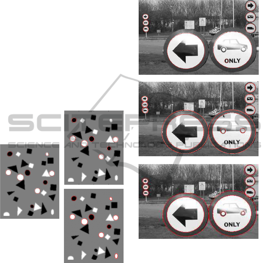
Figure 6: Detected circles superimposed on Test im-

age made of random geometrical dark and bright shapes

(200×250); left: CGC; top right: isophote; bottom right:

EDCircle.

4.2 Application to a Reference Image

The CGC method with the same parameter values (ex-

cept for rmax set to 50) has been used to detect circu-

lar shapes on the image shown in Figure 7 available

http://ceng.anadolu.edu.tr/cv/EDCircles/

where the result of the EDCircle method is also com-

pared to other methods.

Note that the wheels of the car on the right big sign

Figure 7: Detected circles superimposed on Sign Image

(300×198); (top) CGC (middle) Isophote; (bottom) EDCir-

cle.

are detected by the Isophote and EDCircle methods.

The white discs inside the wheels are too small for

the CGC (although it is recommended to use the CGC

with rmin >= 5, if rmin is set to 4, the disc of the left

wheel is detected). The outside circles of the two big

signs are missed by the CGC, as a single circle is as-

sumed at a given location. Only the CGC is detecting

the ”O” of ”only”; even the EDCircle is missing it al-

though it detected shape 26 of Figure 5. Thus, with

respect to sign detection the CGC performs as well as

the best state-of-the-art methods.

4.3 Application to a Satellite Image

The study area is located in the eastern part of

CraterDetectionusingCGC-ANewCircleDetectionMethod

325

Cambodia near the border with Vietnam, in a rural

zone (Choam Kravien) that was heavily bombed dur-

ing the Vietnam War. The terrain is quite ﬂat and

the landscape consists mainly of agricultural land.

The panchromatic image used was acquired by the

WorldView-2 instrument on 26 November 2011. It

covers 100 km

, with a spatial resolution of 0.5 meter

and a pixel depth at acquisition of 11 bits. The method

is used with σ = 1 and δ = 2 for the norm and curva-

ture computation, ε

= ε

= 0.12, t = 10, f = 0.80,

rmin = 5, rmax = 15; only dark circles are detected

and an additional threshold on the circle average norm

is set at t = 50.

The results using our method, isophote and ED-

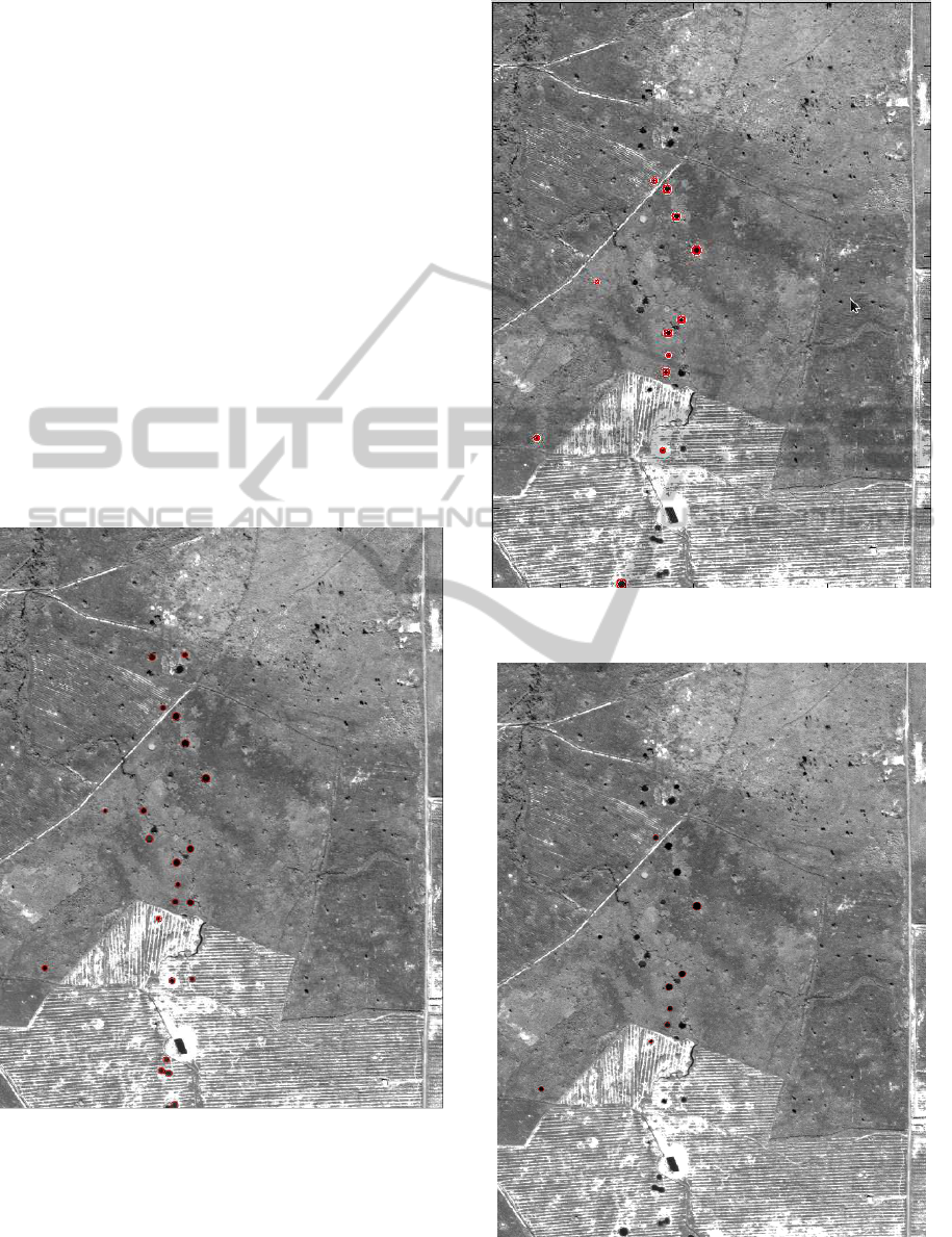
Circles are respectively shown in Figure 8, 9 and 10.

The comparison of the results shows that many

circle shapes are missed by the EDcircle; many are

detected by the isophote method but the CGC method

provide better results. A comparison with visual in-

spection should still be performed to have a quanti-

tative view of the performance of the method in this

context.

Figure 8: Detected circles (CGC) superimposed on

1309×1855 part of the panchromatic image.

Figure 9: Detected circles (Isophote method) superimposed

on 1309×1855 part of the panchromatic image.

Figure 10: Detected circles (EDCircle method) superim-

posed on 1309×1855 part of the panchromatic image.

ICPRAM2015-InternationalConferenceonPatternRecognitionApplicationsandMethods

326

5 DISCUSSION AND

CONCLUSIONS

The Constrained Gradient for Circle (CGC), a

new two-phase method for extracting circles seems

promising. The originality of the method resides in

the ﬁrst phase that uses a gradient angle and curva-

ture compatibility constraint at pixels lying on vari-

ous digital circles to produce sets of connected pixels

belonging to potential circle candidates. The second

phase consists in ﬁnding the best pair of circle-centre

that optimizes the circle position. The method has

been been compared to state-of-the-art methods ap-

plied to an artiﬁcial image, a reference image and a

panchromatic satellite image of Cambodia for crater

detection. The results seem promising. The process

could be performed in parallel, not only at each pixel,

but also for each of the digital circles, which makes

the method efﬁcient. Although the method in the cur-

rent form can deal with any radius range and various

portions of circle, it is better suited to the detection of

full disconnected circles whose radius is small com-

pared to the image size. It could be generalized in or-

der to extract overlapping circles, rings and thin rings

by developing another second phase (thin ring detec-

tion would require a further line detection step as pre-

requisite) and also to detect squares, by adapting the

curvature compatibility constraint.

ACKNOWLEDGEMENTS

Special thanks to Dr. De Marco who processed our

data with his method, and to Dr. Akinlar and Dr.

Topal for their site at

http://ceng.anadolu.edu.tr/cv/EDCircles/except

which allows to process any data with their method.

This research is funded by tthe EC FP7 Security

TIRAMISU Project GA 284747.

REFERENCES

Akinlar, C. and Topal, C. (2013). Edcircles: A real-time

circle detector with a false detection control. Pattern

Recognition, 46.

Atherton, T. J. and Kerbyson, D. J. (1999). Size invari-

ant circle detection. Image and Vision Computing,

17:795803.

Blinn, J. (1996). Jim Blinn’s Corner: A Trip Down

the Graphics Pipeline. Morgan Kaufmann series in

computer graphics and geometric modeling. Morgan

Kaufmann Publishers.

Canny, J. (1986). A computational approach to edge de-

tection. IEEE Trans. on Pattern Anal. and Machine

Intelligence, pages 679–697.

Chung, K.-L., Chen, P.-Z., and Pan, Y.-L. (2009). Speed up

of the edge-based inverse halftoning algorithm using

a ﬁnite state machine model approach. Computers &

Mathematics with Applications, 58(3):484 – 497.

Chung, K.-L., Huang, Y.-H., Shen, S.-M., Krylov, A. S.,

Yurin, D. V., and Semeikina, E. V. (2012). Efﬁcient

sampling strategy and reﬁnement strategy for random-

ized circle detection. Pattern Recognition, pages 252–

263.

Hatﬁeld-Consultants (2014). Uxo predictive modeling in

mmg lxml sepon mine development area. Technical

Report 1791.D6.1, Hatﬁeld consultants, East Lansing,

Michigan.

Marco, T. D., Cazzato, D., Leo, M., and Distante, C. (2014).

Randomized circle detection with isophotes curvature

analysis. Pattern Recognition.

Xu, L., Oja, E., and Kultanen, P. (1990). A new curve de-

tection method: Randomized hough transform (rht).

Pattern Recognition Letters, 11:331338.

Yip, R. K., Tam, P. K., and Leung, D. N. (1992). Modiﬁca-

tion of hough transform for circles and ellipses detec-

tion using a 2-dimensional array. Pattern Recognition,

25:10071022.

Zelniker, E. E. (2006). Maximum-likelihood estimation of

circle parameters via convolution. IEEE Transaction

on Image Processing, 16:865–876.

CraterDetectionusingCGC-ANewCircleDetectionMethod

327