On Error Probability of Search in High-Dimensional Binary Space

with Scalar Neural Network Tree

Vladimir Kryzhanovsky

, Magomed Malsagov

, Juan Antonio Clares Tomas

and Irina Zhelavskaya

Scientific Research Institute for System Analysis, Russian Academy of Sciences, Moscow, Russia

Institute of secondary education: IES SANJE, Alcantarilla, Murcia, Spain

Skolkovo Institute of Science and Technology, Moscow, Russia

Keywords: Nearest Neighbor Search, Perceptron, Search Tree, High-Dimensional Space, Error Probability.

Abstract: The paper investigates SNN-tree algorithm that extends the binary search tree algorithm so that it can deal

with distorted input vectors. Unlike the SNN-tree algorithm, popular methods (LSH, k-d tree, BBF-tree,

spill-tree) stop working as the dimensionality of the space grows (N > 1000). The proposed algorithm works

much faster than exhaustive search (26 times faster at N=10000). However, some errors may occur during

the search. In this paper we managed to obtain an estimate of the upper bound on the error probability for

SNN-tree algorithm. In case when the dimensionality of input vectors is N≥500 bits, the probability of error

is so small (P<10

-15

) that it can be neglected according to this estimate and experimental results. In fact, we

can consider the proposed SNN-tree algorithm to be exact for high dimensionality (N ≥ 500).

1 INTRODUCTION

The paper considers the problem of nearest-neighbor

search in a high-dimensional (N > 1000) configura-

tion space. The components of reference vectors

take either +1 or -1 equiprobably, so the vectors are

the same distance apart from each other and distrib-

uted evenly. We measure the distance between two

points with the Hamming distance. In this case

popular algorithms become either unreliable or

computationally infeasible.

In (Kryzhanovsky, 2013) we investigated the fol-

lowing algorithms: k-dimensional trees (k-d trees)

(Friedman, 1977), spill-trees (Ting, 2004), LSH

(Locality-sensitive Hashing) (Indyk, 1998). We have

found that k-d trees for N > 100 requires one or two

orders of magnitude more computations than ex-

haustive search (BBF-trees (best bin first) (Beis,

1997) were used). As dimensionality N grows, the

error probability of the LSH algorithm approximates

one. In the event when the working point coincides

with a reference, the spill-tree algorithm works fast-

er than the exhaustive search (by an order of magni-

tude), but slower than the binary tree by approxi-

mately five orders of magnitude. The paper exam-

ines the case when the distance between query point

and reference one is greater than 0.1N. In these con-

ditions the spill-tree algorithm is slower than the

exhaustive search and thus its use makes no sense.

In (Kryzhanovsky, 2013) we offered a tree-like

algorithm with perceptrons at tree nodes. Going

down the tree is accompanied with the narrowing of

the search area. The tree-walk continues until the

stop criterion is satisfied. The algorithm works faster

than the exhaustive search even when the dimen-

sionality increases (for example, at N = 2048 it is 12

times faster).

In this paper we estimated the upper bound on

the error probability of the algorithm. The error

probability drops exponentially as the dimensionali-

ty of the problem N grows. For example, at N≥500

the error probability cannot be measured, i.e. the

proposed algorithm can be considered exact in this

range. Thus, the exact algorithm that excels exhaus-

tive search in speed was obtained.

2 PROBLEM STATEMENT

The algorithm we offer tackles the following prob-

lem. Let there be

binary N-dimensional patterns:









,1,1;.

Rx M





X

(1)

300

Kryzhanovsky V., Malsagov M., Clares Tomas J. and Zhelavskaya I..

On Error Probability of Search in High-Dimensional Binary Space with Scalar Neural Network Tree.

DOI: 10.5220/0005152003000305

In Proceedings of the International Conference on Neural Computation Theory and Applications (NCTA-2014), pages 300-305

ISBN: 978-989-758-054-3

 2014 SCITEPRESS (Science and Technology Publications, Lda.)

A binary vector

is an input of the system. It is

necessary to find any reference vector



belonging

to a predefined vicinity of input vector

X . In math-

ematical terms the condition looks like:





max

12 ,bN



XX

(2)

where





max

0; 0.5b 

is a predefined constant that

determines the size of the vicinity.

We will show below that the algorithm solves a

more complex problem from a statistical point of

view: it can find the closest pattern to an input vec-

tor. The Hamming distance is used to determine the

closeness of vectors.

In this paper we consider the case when refer-

ence vectors are bipolar vectors generated randomly.

Generated independently of one another, the compo-

nents of the reference vectors take +1 or -1 with

equal probability (density coding).

3 THE POINT OF THE

ALGORITHM

The idea of the algorithm is that the search area

becomes consecutively smaller as we descend the

tree. In the beginning the whole set of patterns is

divided into two nonoverlapping subsets. A subset

that may contain an input vector is picked using the

procedure described below. The subset is divided

into another two nonoverlapping subsets, and a sub-

set that may contain the input vector is chosen again.

The procedure continues until each subset consists

of a single pattern. Then the input vector is associat-

ed with one of the remaining patterns using the same

procedure.

The division of the space into subsets and the

search for a set containing a particular vector can be

quickly done using a simple perceptron with a “win-

ner takes all” decision rule. Each set is controlled by

a perceptron trained on the patterns of corresponding

subset. Each output of the root perceptron points to a

tree node of the next level. The perceptron of the

descendant node is trained on a subset of patterns

corresponding to one output of the root perceptron.

The descent down a particular branch of the tree

brings us to a pattern that can be regarded as a solu-

tion. At each stage of the descent we pick a branch

that corresponds to the perceptron output with the

highest signal. It is important to note that the same

vector

is passed to each node rather than the result

of work of the preceding-node perceptron.

4 THE PROCESS OF LEARNING

Each node of the tree is trained independently on its

own subset of reference points. A root perceptron of

the tree is trained on all

patterns. Each descend-

ent of a root node is trained on

2M patterns. The

nodes of the i-th layer are trained on



pat-

terns,

1, 2, ; logikkM



 is the number of lay-

ers in the tree.

All nodes have the same structure – a single-

layer perceptron (Kryzhanovsky, 2010) that has

input bipolar neurons and two output neurons each

of which takes one of the three values





1, 0, 1 , 1, 2

yi  

Let us consider the operation of one node using a

root element as an example (all nodes are identical

to each other). The Hebb rule is used to train the

perceptron:







WYX

(3)

where

is a 2 N



-matrix of synaptic coefficients,

and



is a two-dimensional vector that defines the

required response of the perceptron to the



-th

reference vector



X .



may take one of the follow-

ing combinations of values: (-1,0), (+1,0), (0,-1), and

(0,+1). If the first component of



is nonzero, the

reference vector



is assigned to the left branch.

Otherwise, it is assigned to the right branch. Since

the patterns are generated randomly (and therefore

distributed evenly), the way they are divided into

subsets is not important. The set of patterns is al-

ways divided into two equal portions corresponding

to the left and right branches of the tree during the

training so that the four possible values of



should

be distributed evenly among all patterns, i.e.







Y .

The perceptron works in the following way. The

signal on output neurons is first calculated:

.hWX

(4)

Then the “winner takes all” criterion is used: a

component of vector h with the largest absolute

value is determined. If it is the first component, the

reference vector should be sought for in the left

branch, otherwise in the right branch.

The number of operations needed to train the

whole tree is

2log.





(5)

OnErrorProbabilityofSearchinHigh-DimensionalBinarySpacewithScalarNeuralNetworkTree

301

5 THE SEARCH ALGORITHM

Before we start describing the search algorithm, we

should introduce a few notions concerning the algo-

rithm.

Pool of losers. When vector X is presented to a

perceptron, it produces certain signals at the outputs.

An output that gives the largest signal is regarded as

a winner, the others as losers. The pool of losers

keeps the value of the output-loser and the location

of the corresponding node.

Pool of responses. After the algorithm comes to

a solution (tree leaf), the number of a pattern associ-

ated with the leaf and the value of the output signal

of a perceptron corresponding to the solution are

stored in the pool of responses. So each pattern has

its leaf in the tree.

Search stopping criterion. If the algorithm comes

to a tree leaf and the signal amplitude becomes

greater than a threshold value, the search stops. It

means that condition (2) holds.

Location of a node is a unique identifier of the

node.

Descending the tree is going down from one

node to another until the leaf is reached. The branch-

ing algorithm is as follows:

1. The input neurons of a perceptron associated with

a current tree node are initiated by input vector

. Output signals of the perceptron

h and

are calculated.

2. The output with the highest signal and the de-

scendent node related to this output (descendent-

winner) are determined. The signal value of the

loser output and location of the corresponding de-

scendent-node are stored in the pool of losers.

3. If a tree leaf is reached, go to step 5, otherwise to

step 4.

4. Steps 1 to 4 are repeated for the descendent-

winner.

5. The result is put in the pool of responses. At this

point the branching algorithm stops.

Now we can formulate our algorithm. Process of

descending different tree branches is repeated until

the stopping criterion is met. The stages of the algo-

rithm are:

1. We descend the tree from the root node to a leaf.

The pool of losers and pool of responses are filled

in during the process.

2. We check the stopping criterion (2) for the leaf,

i.e. we check if the scalar product of vector

and the pattern related to the leaf is greater than a

predefined threshold. If the criterion is met, we go

to step 4, otherwise to step 3.

3. If the criterion fails, we pick a node with the

highest signal amplitude from the pool of losers

and repeat steps 1 to 3 starting the descend from

this node now.

4. We pick a pattern with the highest signal value in

the pool of responses, and regard it as a solution.

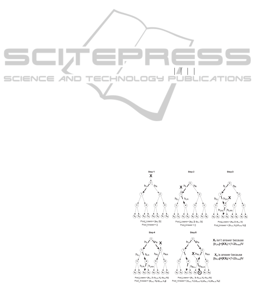
6 EXAMPLE OF THE

ALGORITHM OPERATION

Let us exemplify the operation of the algorithm.

Figure 1 shows a step-by-step illustration of the

algorithm for a tree built for eight patterns





Step 1: the tree root (node 0) receives input vector

. The root perceptron generates signals

h and

at its outputs. Let

hh

, then

h and the loca-

tion of the descendant-node connected to the right

output (node 2) are placed in the pool of losers. Step

2: vector

is fed to the node-winner (node 1). A

winning node is determined again and the loser is

put in the pool (e.g.

h and node 3). Step 3: after

reaching the leaves, we put patterns (

and

X )

associated with the leaves and signal values

3LRL



XX and

4LRR



XX in the pool of respons-

es. Then we check if the patterns meet criterion (2).

In our case the criterion is not met, so the algorithm

continues its work. Step 4: if none of the patterns

satisfies the solution, we pick the highest-signal

node from the pool of losers (for example, node 2

Figure 1: An example of the algorithm operation.

NCTA2014-InternationalConferenceonNeuralComputationTheoryandApplications

302

with signal

h ). Step 5: now the descent starts from

this node (node 2) and continues until we reach the

leaves while the pool of losers taking new elements.

At that pair



h is moved away from the pool of

losers. Here

LL RLR

hh

and



max

bNh

i.e. criterion (2) is true for pattern

X . The pattern

becomes the winner and the algorithm stops. If the

criterion never works during the operation of the

algorithm, the pattern from the pool of responses

with the highest signal value is regarded as winner.

7 ESTIMATION OF THE ERROR

PROBABILITY

It is hard to obtain a precise estimate of the error

probability for the proposed algorithm as for now.

However, it is possible to get its upper bound.

SNN-tree algorithm can fail in case when there is

more than one pattern that satisfies criterion (2) in

the set. Formally, the probability of this event can be

written as:

max

1Pr (12 ) .

PbN







  







(6)

Presence of such patterns does not always lead to

the algorithm failure. Therefore, probability (6) can

be used as an estimation of the upper bound on the

proposed algorithm failure.

Equation (6) can be calculated exactly by formu-

la:

max

11 .







 







(7)

However, it is not possible to use formula (7) at

large values of N (N>200). For high dimensions, it is

better to use approximation:

exp













max

(1 2 ) .NN b



(8)

Equation (8) shows that the error probability ex-

ponentially decreases as the problem dimensionality

N grows. For example, at N=500 and b

max

=0.3 power

of the exponent is -40, which explains the fact that

experimental error probability for high dimensions

could not be measured in work (Kryzhanovsky,

2014). In fact, SNN-tree can be considered exact for

high dimensional problems.

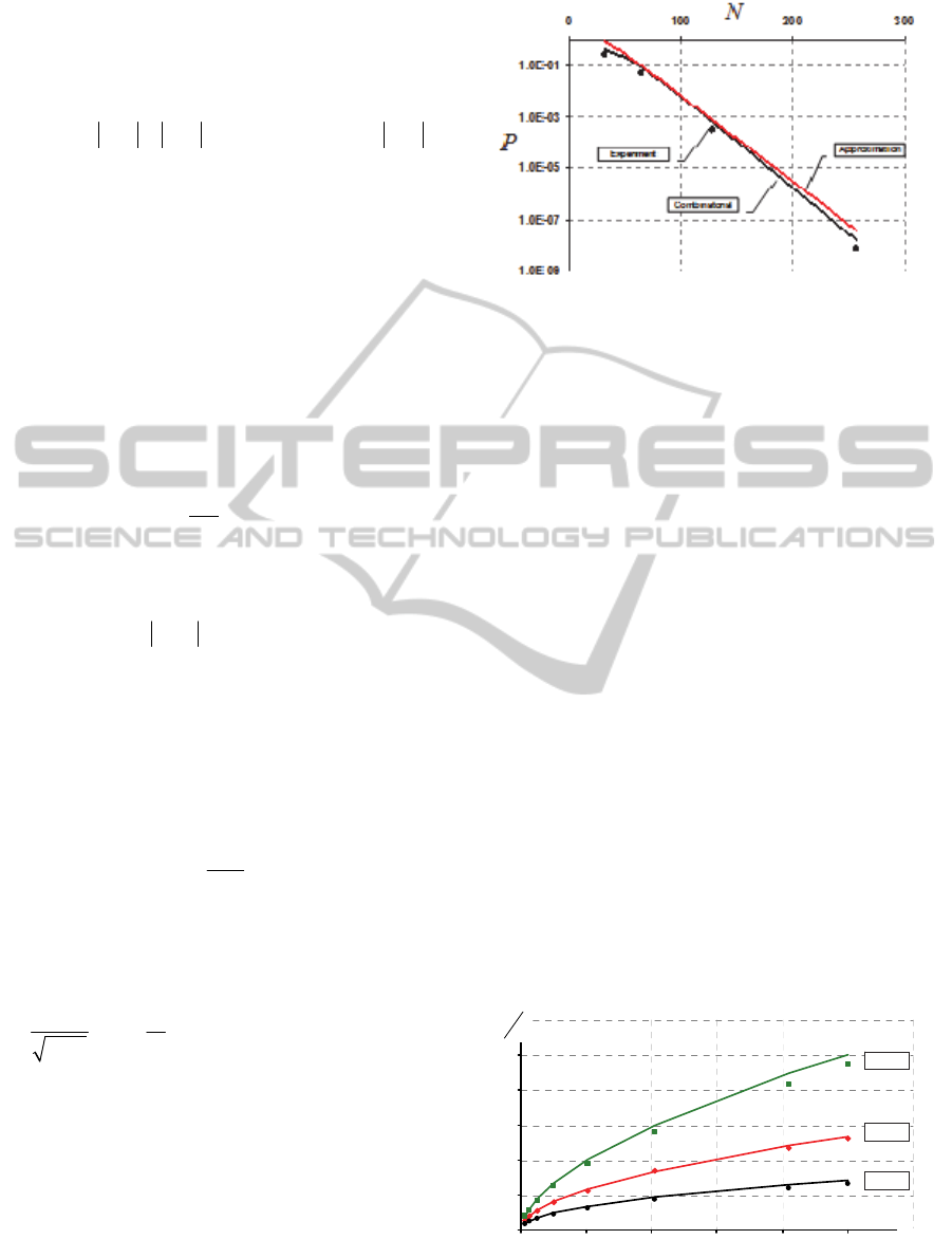
Figure 2 shows dependence of the error probabil-

ity on dimensionality N at b

max

=0.3 and M=N. As

Figure 2: The algorithm error probability.

expected, the error probability of the algorithm

(markers) is smaller than probabilities calculated

using (7) and (8) (solid lines). Therefore, expres-

sions (7) and (8) can be used for algorithm reliability

estimation. Moreover, it can be seen that expression

(8) is a sufficient approximation of (7).

8 ESTIMATION OF THE

COMPUTATIONAL

COMPLEXITY

Estimation of the proposed algorithm computational

complexity is a quite sophisticated problem that was

not solved yet. In this section, results of computa-

tional modeling are presented.

It was shown in work (Kryzhanovsky, 2014) that

the problem in hand could be solved using only

these two algorithms: exhaustive search and SNN-

tree. Conducted research shows that the proposed

algorithm works faster than exhaustive search, how-

ever it errors may occur. According to the results

from the previous sections, the error probability at

dimensionality N≥500 is so small that it can be ne-

glected. Therefore, even a small speed advantage of

SNN-tree over exhaustive search makes it prefera-

ble.

0 2000 4000 6000 8000 10000 12000

b = 0.3

b = 0.2

b = 0.1



Figure 3: The speed advantage of SNN-tree over exhaus-

tive search (markers - experiment; solid lines – estima-

tion).

OnErrorProbabilityofSearchinHigh-DimensionalBinarySpacewithScalarNeuralNetworkTree

303

Experiments show (Fig. 3) that as dimensionality N

grows the speed advantage of SNN-tree over ex-

haustive search increases. For example, at

N=M=2 000 and b=0.2 SNN-tree is faster than ex-

haustive search in 12 times, and at N=M=10 000

acceleration reaches 26 times. Note b

max

is a fixed

value, but b is a number of distorted components in

the input vector. Using experimental result, we esti-

mated the average number of scalar product opera-

tions needed for SNN-tree search:







exp 1.3 0.44 0.4 log .

bbN





(9)

Solid lines in figure 3 were built using equation

(9). This equation allows estimating average speed

advantage of SNN-tree over exhaustive search. Us-

ing (9), it is possible to predict advantage of SNN-

tree at large values of parameters (table 1).

Table 1: The speed advantage of SNN-tree over exhaus-

tive search for M=N=10

and b

max

=0.3 using equation (9).

b M / θ

0.1 189

0.2 88

0.3 41

9 CONCLUSIONS

The paper considers the problem of nearest-neighbor

search in a high-dimensional configuration space.

The use of most popular methods (k-d tree, spill-

tree, BBF-tree, LSH) proved to be inefficient in this

case. We offered a tree-like algorithm that solves the

given problem (SNN-tree).

In this work, theoretical estimate of the upper

bound on the error probability of SNN-tree algo-

rithm was obtained. This estimate shows that the

error probability decreases as the dimensionality of

the problem grows. Since even at N>500 the error is

less than 10

-15

, it does not seem possible to measure

it experimentally. Therefore, it is safe to say that

SNN-tree is an exact algorithm. Research investiga-

tions of the computational complexity of the algo-

rithm shows that the speed advantage of SNN-tree

algorithm over exhaustive search increases as the

dimensionality N grows.

So, we can conclude that SNN-tree algorithm

represents an efficient alternative to exhaustive

search.

ACKNOWLEDGEMENTS

The research is supported by the Russian Foundation

for Basic Research (grant 12-07-00295a).

REFERENCES

Friedman, J.H., Bentley, J.L. and Finkel, R.A., 1977.An

algorithm for finding best matches in logarithmic ex-

pected time. ACM Transactions on Mathematical

Software. vol. 3. pp. 209–226.

Ting Liu, Andrew W. Moore, Alexander Gray and Ke

Yang., 2004. An Investigation of Practical Approxi-

mate Nearest Neighbor Algorithms. Proceeding of

Conference. Neural Information Processing Systems.

Indyk, P. and Motwani, R., 1998. Approximate nearest

neighbors: Towards removing the curse of dimension-

ality. In Proc. 30

STOC. pp. 604–613.

Beis, J.S. and Lowe, D.G., 1997. Shape Indexing Using

Approximate Nearest-Neighbor Search in High-

Dimensional Spaces. Proceedings of IEEE Computer

Society Conference on Computer Vision and Pattern

Recognition. pp. 1000-1006.

Kryzhanovsky B., Kryzhanovskiy V., Litinskii. L., 2010.

Machine Learning in Vector Models of Neural Net-

works. // Advances in Machine Learning II. Dedicated

to the memory of Professor Ryszard S. Michalski. Ko-

ronacki, J., Ras, Z.W., Wierzchon, S.T. (et al.) (Eds.),

Series “Studies in Computational Intelligence”.

Springer. SCI 263, pp. 427–443.

Kryzhanovsky V., Malsagov M., Tomas J.A.C., 2013.

Hierarchical Classifier: Based on Neural Networks

Searching Tree with Iterative Traversal and Stop Cri-

terion. Optical Memory and Neural Networks (Infor-

mation Optics). vol. 22. No. 4. pp. 217–223.

Kryzhanovsky V., Malsagov M., Zelavskaya I., Tomas

J.A.C., 2014. High-Dimensional Binary Pattern Clas-

sification by Scalar Neural Network Tree. Proceedings

of International Conference on Artificial Neural Net-

works. (in print).

APPENDIX A

It is necessary to calculate the following probability:

max

1Pr (12 ) .

PbN









  











(А1)

Let scalar products

XX and



be inde-

pendent random quantities,





max

1Pr (12).

PbN





 







(А2)

NCTA2014-InternationalConferenceonNeuralComputationTheoryandApplications

304

Now, it is necessary to calculate the probability that

the product of each pattern by input vector is smaller

than the threshold.

Scalar product

XX is a discrete quantity, which

values lie in

[;]NN

. Let k be the number of com-

ponents with the opposite sign in vectors

and

X . Then its probability function is:



Pr ( 2 ) .

Nk XX

(А3)

Random variable

XX is symmetrically distrib-

uted with zero mean, so

max

Pr (1 2 ) 1 2 .



 





(А4)

From А2 and А4 we can conclude that

max

112 .







 







(А5)

APPENDIX B

Scalar product

mimi









(B1)

consists of a large number of random quantities.

Therefore, at big dimensions (N>100) its distribution

can be approximated by Gaussian law with the fol-

lowing probability moments:



 и









(B2)

Therefore, probability (А1) can be described by

integral expression:

max

(1 2 )

~1 1 .

Ped



























(B3)

Using the following approximation

,1,

edt x











(B4)

obtain the final estimation of probability (А1.1):

exp













max

(1 2 ) .NN b



(B5)

OnErrorProbabilityofSearchinHigh-DimensionalBinarySpacewithScalarNeuralNetworkTree

305