
Proactive Evolutionary Algorithms for Dynamic Optimization Problems
Patryk Filipiak
Computational Intelligence Research Group, Institute of Computer Science, University of Wroclaw, Wroclaw, Poland
1 STAGE OF THE RESEARCH
The research is ongoing for nearly four years. The
preliminary results and possible applications were
presented on 6 international conferences and pub-
lished in 10 papers available in: Lecture Notes in
Computer Science (Filipiak et al., 2011; Filipiak et al.,
2012a; Filipiak et al., 2012b; Michalak et al., 2013;
Filipiak and Lipinski, 2014a; Filipiak and Lipinski,
2014b; Lancucki et al., 2014; Michalak et al., 2014),
Lecture Notes in Artificial Intelligence (Filipiak and
Lipinski, 2012) and Lecture Notes in Mechanical En-
gineering (Brzychczy et al., 2014) by Springer.
A completion of the PhD thesis is planned for the
academic year 2014/2015.
2 OUTLINE OF OBJECTIVES
The aim of the research is to propose the anticipa-
tion strategies that are easily applicable to the contem-
porary Evolutionary Algorithms in order to improve
their robustness in dealing with Dynamic Optimiza-
tion Problems (defined in the next section).
A thorough examination of the suggested ap-
proach and the classification of optimization prob-
lems that are solvable with it are necessary to fill the
research gap in this area.
Eventually, a comparison of the introduced algo-
rithms with the state-of-the-art solutions, both reac-
tive and proactive, needs to be done.
3 RESEARCH PROBLEM
Numerous real-world optimization problems are dy-
namic in a sense that their objective functions change
as time goes by which makes them difficult to solve.
Such dynamic objective function can be defined by
F
(α
t
)
: R
d
−→ R, (1)
where d > 0 and (α
t
) is a vector of parameters chang-
ing in time, indexed with t ∈ T ⊆ N.
A solution to Dynamic Optimization Problem
(DOP) is a set of pairs S = {(x,t) : x ∈ R
d
, t ∈ T},
where for all (x,t) ∈ S holds
x = arg min{F
(α
t
)
(x) : x ∈ R
d
}. (2)
In other words, solving DOPs is not only about find-
ing the biggest peak in the landscape yet also about
tracking its movement and continuously exploring the
search space looking for the newly appearing optima.
It has to be clarified that the vector of parame-
ters (α
t
) is not known for all t ∈ T . Let t
now
∈ T
encode the present moment which implies that only
(α
t
now
) can currently be observed. It is often assumed
that vectors (α
t
)
t∈T
for t < t
now
can also be accessi-
ble since one is usually able to keep the record of past
observations (e.g. stock quotes, weather conditions)
or events (e.g. alerts, system log files). However, the
future values (α
t
)
t∈T
for t > t
now
clearly cannot be
accessible until the t increases.
The above-defined DOPs are present in a wide
range of academic and engineering fields, e.g. time
series analysis (Box et al., 2011), decision support
systems (Kim, 2006), inverse kinematics (Castellani
and Fahmy, 2008), job scheduling and load balancing
tasks (Jozefowiez et al., 2009).
3.1 Evolutionary Approach
Evolutionary Algorithms (EAs) are a class of easily
applicable, self-adaptive heuristic optimization prob-
lem solvers that allow for a fast exploration of large
parameter spaces aiming to find the (at least) sub-
optimal solutions. Even though EAs were origi-
nally designed for Stationary Optimization Problems
(SOPs), their adaptation to the DOPs domain is rather
straightforward (Branke, 2001). In the commonly
used reactive model EAs probe for the landscape
changes by triggering some simple actions in the syn-
chronous manner, e.g. a re-evaluation of certain in-
dividuals in the population or a random sampling of
the search space. Immediately after a change of the
objective function is detected, a dedicated procedure
aimed at localizing new optima is launched.
The main drawback of the above model is its iner-
tia. Note that reactive EAs are always one step behind
3
Filipiak P..
Proactive Evolutionary Algorithms for Dynamic Optimization Problems.
Copyright
c
2014 SCITEPRESS (Science and Technology Publications, Lda.)

the changing environment since they can only respond
to the changes that were already detected, providing
that they were detected at all.
3.2 Improvement Due to Proactivity
A proactive model aims at acting a priori rather than
a posteriori. It collects the past observations of the
changing environment and utilizes them to anticipate
the future landscape. This way, the EA can deal in
advance with the changes to come, for instance by
directing a part of the population towards the most
probable future promising regions.
Although in theory the proactive model clearly
seems much more robust then the reactive one, it is
generally hard to achieve in practice since no antici-
pation mechanism can be fully reliable. Thus, a fun-
damental research problem is to propose a class of
the forecasting models that the EAs can be equipped
with and to analyze the applicability of the proposed
proactive EAs to the certain types of DOPs.
Eventually, it has to be verified whether the sug-
gested proactive algorithms indeed outperform the re-
active ones as it is assumed in the theoretical model,
and if so, then what is the obtained speed up.
4 STATE OF THE ART
Most EAs applied for SOPs follow the same two-
stage pattern. They begin with the low-grained ex-
ploration of the search space aimed at localizing the
most promising regions and then gradually switch to
the exploitation stage when a fine-grained search is
performed. Nevertheless, the above behaviour does
not comply with DOPs. In the case of continuously
changing environment both exploration and exploita-
tion are carried on simultaneously since EA, during
whole its run, has to probe for the new optima in par-
allel with tracking the ones that were already found.
Otherwise, the population would soon converge to
a small neighbourhood of some local optimum and
thus immediately lose the ability to detect new optima
emerging outside this neighbourhood.
4.1 Introducing Diversity
A number of EAs proposed by the researchers to ad-
dress DOPs aim at forcing a diversification among
tightly coupled individuals. Cobb proposed a Trig-
gered Hypermutation (TH) mechanism that activates
whenever a moving average of best individuals fitness
deteriorates. The mutation rate is then increased to the
predefined high level so that the individuals could be
spread evenly across the search space (Cobb, 1990).
An improved TH mechanism named Variable Local
Search (VLS) was suggested in (Vavak et al., 1997).
It performs a gradual increasing and decreasing of the
mutation rate (rather than switching sharply between
the two fixed levels) which improves the performance
of VLS in DOPs with low severity of changes.
An alternative approach to diversifying the pop-
ulation on a triggered basis is to maintain a certain
level of diversity throughout the whole run of EA. A
popular Genetic Algorithm (GA) of this type, named
Random Immigrants GA (RIGA), was first introduced
in (Grefenstette, 1992). Near the end of each genera-
tion it selects a small fraction of individuals to replace
them with the purely random ones. As a result a bunch
of mediocre individuals is obtained each time yet the
search space is relatively well covered and, what is
more, there is no need for the environmental change
detector. Another method for maintaining diversity
was implemented in CHC (Sim
˜
oes and Costa, 2011),
where only sufficiently distant individuals (in terms
of a Hamming distance) are allowed for mating and
crossing-over in order to prevent them from incest.
4.2 Memory Based Approach
In DOPs with periodical or recurrent changes it is of-
ten convenient to store the historical best solutions so
that they can be re-used afterwards when the environ-
ment reaches the same state again. One possible ap-
proach to achieve this is through polyploidy, i.e. a col-
lection of multiple information about each allel in the
chromosome (Yang, 2006). Such chromosome is then
additionally equipped with the adaptive mask that in-
dicates which of the redundant allels dominates the
others that are kept in the same locus. This way one
genotype may encode various phenotypes depending
on the current state of the adaptive mask.
The algorithms using memory explicitly were also
proposed. A direct use of the previous good solutions
stored in a buffer was well studied in (Yang, 2005).
Alternatively, some indirect strategies for the use of
a memory were suggested that either collect states of
the environment (Eggermont et al., 2001), a probabil-
ity vector that created best individuals (Yang and Yao,
2008) or a likelihood that an optimum would appear
in a certain area (Richter and Yang, 2008).
4.3 Proactivity
Prediction approaches to DOPs are still not well stud-
ied. A “futurist” mechanism that empowered Sim-
ple GA (SGA) by directing the population into the fu-
ture promising regions was signalized in (van Hemert
IJCCI2014-DoctoralConsortium
4

et al., 2001) yet the author considered only the per-
fect predictor. A number of true anticipation mod-
els based on Kalman filter (Rossi et al., 2008), auto-
regression (Hatzakis and Wallace, 2006) or time se-
ries identification (Zhou et al., 2007) were proposed
to address some specific DOPs. An interesting ap-
proach using an auto-regressive model for predicting
when the next change will occur and a Markov chain
predictor for anticipating the future landscape was re-
cently presented in (Sim
˜
oes and Costa, 2013). The
latter approach was tested on the popular bit-string
problems where it proved its rapidness in reacting to
the recurring changes.
5 METHODOLOGY
A fundamental part of the research comprises of the
three predictive strategies proposed for EAs so that
they follow the proactive model in solving DOPs.
The first two strategies utilize the Auto-Regressive
Integrated Moving Average model (ARIMA) (Box
et al., 2011) frequently used in statistics and data anal-
ysis. Both of them focus on certain vectors of the
search space that are somehow representative for the
present landscape. The historical data associated to
these vectors is collected in the form of time series.
Later on, the ARIMA model is used for anticipating
the future values of the time series so that EA can
prepare for the next change of the environment that
is likely to happen very soon. The strategies were
employed in Infeasibility Driven Evolutionary Algo-
rithm (IDEA) (Singh et al., 2009a) that, apart from
dealing with DOPs, can also handle constraints which
is a valuable asset in the field of real-world optimiza-
tion problems (see: Appendix).
The third strategy is an extension of the antici-
pation mechanism based on a Markov chain predic-
tor presented in (Sim
˜
oes and Costa, 2013). It makes
a use of the ability of Univariate Marginal Distribu-
tion Algorithm (UMDA) (Liu et al., 2008) to build a
probability model for distribution of good individu-
als within the search space. These models are further
used as the parametrization of the states of the envi-
ronment identified by the anticipation mechanism.
Detailed descriptions of the above strategies are
given in the next sections accompanied with the pre-
liminary results and indications of the future work.
5.1 Anticipation of Evaluations
In this anticipation strategy a dynamism of the en-
vironment is perceived through the recurrent evalu-
ations of a finite set of samples S ⊂ R
d
, d > 0. Every
Algorithm 1: Pseudo-code of IDEA-ARIMA.
S
1
=
/
0
P
1
= RandomPopulation()
Evaluate(P
1
)
for t = 1 → N
gen
do
if the function F has changed then
Re-evaluate(P
t
)
S
t
= ReduceSamples(S
t
∪ P
t
)
Re-evaluate(S
t
\ P
t
)
if t − 1 > N
train
then
P
t
= ReducePopulation(P
t
∪
e
P
t
)
end if
end if
P
t+1
= IDEA
t
(P
t
,F
(t)
)
if t > N
train
then
e
P
t+1
= RandomPopulation()
e
P
t+1
= IDEA
1
(
e
P
t+1
,
e
F
(t+1)
)
end if
S
t+1
= S
t
end for
sample s ∈ S is associated with the time series of its
past evaluations (X
s
t
)
t∈T
, i.e.
∀
t≤t
now
X
s
t
= F
(t)
(s). (3)
In other words, all the historical values of the ob-
jective function F for all the samples s ∈ S up to
the present moment t
now
∈ T are collected and made
available at any time.
The ARIMA model is applied for predicting the
future values of the objective function
e
X
s
t
now
+1
=
e
F
(t
now
+1)
(s) based on the past observations (X
t
)
t≤t
now
.
Then, the whole future landscape can be anticipated
by extrapolating the set
{
e
F
(t
now
+1)
(s); s ∈ S}, (4)
using the k > 0 nearest neighbours method.
The above strategy was applied in IDEA and intro-
duced as IDEA-ARIMA (Filipiak et al., 2011). The
proposed algorithm maintains two concurrent popula-
tions P and
e
P. The first one is responsible for optimiz-
ing the objective function F while the latter optimizes
the anticipated objective function
e
F.
Algorithm 1 presents the pseudo-code of IDEA-
ARIMA. It begins with a random initialization of the
population P
1
and the empty set of samples S
1
. Then
the main loop of the algorithm is run for N
gen
> 0 gen-
erations. Whenever a change of the objective function
F is detected (i.e. the evaluation of at least one of the
randomly chosen individuals has just changed), the
whole population P
t
is re-evaluated and then added
to the set of samples S
t
. After that, the set S
t
is
reduced to the fixed maximum size and the rest of
ProactiveEvolutionaryAlgorithmsforDynamicOptimizationProblems
5

Table 1: Numbers of matches in 10 runs of IDEA and IDEA-ARIMA for benchmarks G24 1 and G24 2 with N
gen
= 64. The
first N
train
= 16 iterations were omitted since observable results of both algorithms do not differ within this time period.
G24 1 G24 2
IDEA 21 23 13 19 19 15 22 16 22 21 5 9 19 10 9 14 11 12 18 14
IDEA-ARIMA 28 26 29 30 28 26 29 29 29 26 29 25 21 23 26 26 23 23 23 22
the samples S
t
\ P
t
is also re-evaluated. Providing
that the training period of the anticipation mechanism
t = 1,2, ... , N
train
is over, and thus the population
e
P
t
is ready, the individuals from P
t
and
e
P
t
are grouped
together and immediately reduced to the fixed popu-
lation size M > 0. Eventually, regardless the changes
of F, the t-th iteration of the original IDEA is invoked.
Later on, the predictive population
e
P
t+1
is initialized
randomly and used for the one iteration of IDEA with
the anticipated objective function
e
F
(t+1)
.
IDEA-ARIMA was tested on the dynamic con-
strained benchmark problems from the G24 family
(Nguyen and Yao, 2009a) and the modified FDA1
(Farina et al., 2004; Filipiak et al., 2011). Figure 1
present the 2D-plots of the objective functions and
their anticipated counterparts at the sample time steps.
Darker shades represent lower values of F
(t)
. It is
clear that although the anticipations are not exact in
every point of the search space, the promising regions
(marked in black) are well identified.
Table 1 summarizes the numbers of matches (i.e.
correct identifications of global optimum among local
ones) at each time step N
train
< t ≤ N
gen
of G24 1 and
G24 2 benchmark problems. An identification was
(a) Benchmark G24 1
0 0.5 1 1.5 2 2.5 3
0
0.5
1
1.5
2
2.5
3
3.5
4
0 0.5 1 1.5 2 2.5 3
0
0.5
1
1.5
2
2.5
3
3.5
4
F
(25)
e
F
(25)
seen at t = 24
(b) Benchmark mFDA1
0 0.1 0.2 0.3 0.4 0.5 0.6 0.7 0.8 0.9 1
−1
−0.8
−0.6
−0.4
−0.2
0
0.2
0.4
0.6
0.8
1
0 0.1 0.2 0.3 0.4 0.5 0.6 0.7 0.8 0.9 1
−1
−0.8
−0.6
−0.4
−0.2
0
0.2
0.4
0.6
0.8
1
F
(18)
e
F
(18)
seen at t = 17
Figure 1: 2D-plots of the objective functions (left) and
their counterparts anticipated with IDEA-ARIMA (right)
at the sample time steps of benchmarks: (a) G24 1 and
(b) mFDA1. Darker shades represent lower values of F
(t)
.
considered correct whenever the Euclidean distance
between the global optimum and at least one feasible
solution did not exceed δ = 0.1. It is easy to see that
IDEA-ARIMA outperformed IDEA in each run.
Finally, it has to be mentioned that IDEA-ARIMA
was tested with no limitations on the size of the set of
samples S (maximum size set to ∞). In the future an
effective reduction mechanism on the set S ought to be
proposed. Also the number of historical evaluations
stored in time series needs to be limited due to the
excessive memory usage.
5.2 Anticipation of Optima Locations
The second approach is an extension of the Feed-
forward Prediction Strategy (FPS) proposed in
(Hatzakis and Wallace, 2006). It assumes that the
changes of spatial locations of optima inside the
search space form a pattern that can be fitted with an
AutoRegressive (AR) model. As a result, the loca-
tion of future optimum can be anticipated using this
model.
For all time steps t ∈ T , let x
∗
t
∈ R
n
be the argu-
ment minimizing F
(t)
, i.e. the location of optimum of
F
(t)
. Let {X
t
}
t∈T
be the n-dimensional time series of
such optima locations, i.e. X
1
= x
∗
1
, X
2
= x
∗
2
,.. . Ob-
viously, the exact values of x
∗
t
aren’t known. Instead,
an individual p
∗
t
∈ R
n
with the highest fitness among
all specimens in a population P
t
at time step t is used
as the best available approximation of x
∗
t
. As a result,
the accuracy of a prediction model is highly depen-
dent on the efficiency of the EA used. It means that
the closer a population can get to the actual optimum
at each time step, the more exact locations of future
optima can be anticipated. On the other hand, the less
effectively EA performs at localizing current optima,
the more erroneous anticipations it obtains in return.
The original FPS was based on a simple AR model
parametrized with only a single positive integer deter-
mining the order of autoregression. In the proposed
approach, the AR is extended into the more general
ARIMA model that often guarantees more accurate
forecasts. The suggested extension of FPS was ap-
plied to IDEA and introduced as IDEA-FPS (Filipiak
and Lipinski, 2014a).
Apart from the prediction mechanism, IDEA-FPS
provides a novel population segmentation on explor-
ing, exploiting and anticipating fractions.
IJCCI2014-DoctoralConsortium
6
Algorithm 2: Pseudo-code of IDEA-FPS.
X
0
= (
/
0)
P
1
= RandomPopulation()
for t = 1 → N
gen
do
Evaluate(P
t
)
P
t
= InjectExploringFraction(P
t
,size
explore
)
P
0
t
= IDEA
t
(P
t
,F)
p
∗
t
= BestIndividual(P
0
t
)
X
t
= (X
t−1
,{p
∗
t
})
if t > N
train
then
e
p
∗
t+1
= AnticipateNextBestIndividual(X
t
)
Φ
t+1
= N (
e
p
∗
t+1
,σ
2
t
)
P
t+1
= InjectAnticipatingFraction(P
0
t
,
Φ
t+1
,size
anticip
)
else
P
t+1
= P
0
t
end if
end for
Exploring fraction is built up entirely with ran-
dom immigrants that are uniformly distributed in the
search space. Their randomness prevents a popula-
tion from trapping into local optima and introduces
diversity required for tracking changes in the land-
scape. Anticipating fraction is a group of individu-
als gathered in the nearest proximity of the predicted
location of a future optimum. Providing that a fore-
cast obtained with an anticipation model is accurate,
these individuals become the most contributing ones
just after the next environmental change. Exploiting
fraction in turn is formed with offsprings of explor-
ing and anticipating individuals from previous gener-
ations. It is responsible for a fine-grained search in
the promising regions localized by other fractions.
A pseudo-code of IDEA-FPS is given in Algo-
rithm 2. It begins with a random initialization of M >
0 individuals x
1
,.. . ,x
M
∈ R
d
and the empty time se-
ries {X
t
}
t∈N
. Each iteration t = 1,.. . ,N
gen
starts with
the evaluation of a population P
t
. Later on, a new ex-
ploring fraction comprising of size
explore
· M random
immigrants (where size
explore
∈ {0%, . .., 100%}) is
injected into P
t
. These immigrants replace worst in-
dividuals in P
t
. Next, the t-th iteration of IDEA is
invoked and after that a best-of-population individual
p
∗
t
is selected. A vector p
∗
t
∈ R
d
is then stored in {X
t
}
as the best approximation of an optimum location at
time step t.
For t = 1,. . .,N
train
the anticipation mechanism
of IDEA-FPS is inactive since best individuals from
these generations are used for training the ARIMA
model. During this initial period IDEA-FPS behaves
like the original IDEA extended with random immi-
grants injections.
When the condition t > N
train
is finally satis-
(a) Benchmark G24 1
32 33 34 35 36 37 38 39 40 41 42 43 44 45 46 47 48
−6
−4
−2
0
generation number
min eval.
IDEA
32 33 34 35 36 37 38 39 40 41 42 43 44 45 46 47 48
−6
−4
−2
0
generation number
min eval.
IDEA with restart
32 33 34 35 36 37 38 39 40 41 42 43 44 45 46 47 48
−6
−4
−2
0
generation number
min eval.
IDEA−FPS
(b) Benchmark mFDA1
32 33 34 35 36 37 38 39 40 41 42 43 44 45 46 47 48
0
0.1
0.2
0.3
0.4
generation number
min eval.
IDEA
32 33 34 35 36 37 38 39 40 41 42 43 44 45 46 47 48
0
0.1
0.2
0.3
0.4
generation number
min eval.
IDEA with restart
32 33 34 35 36 37 38 39 40 41 42 43 44 45 46 47 48
0
0.1
0.2
0.3
0.4
generation number
min eval.
IDEA−FPS
Figure 2: Comparison of the evaluations of best individuals
during a sample run of IDEA-FPS vs. IDEA and IDEA with
restart, tested in G24 1 and mFDA1.
fied, ARIMA is applied to {X
t
} in order to obtain a
forecast concerning the next optimum location
e
p
∗
t+1
.
As a result, the new anticipation fraction is created
out of random individuals located in the proximity
of
e
p
∗
t+1
. Virtually any continuous probability dis-
tribution function can be applied for that purpose.
In the proposed approach the anticipation fractions
are drawn with a d-dimensional Gaussian distribu-
tion N (
g
p
∗
t+1
,σ
2
t
) where σ
t
= (σ
t,1
,σ
t,2
,.. . ,σ
t,d
) ∈ R
d
with σ
t,i
= (x
max
i
− x
min
i
)/100t for i = 1, ... ,d and
x
min
i
≤ x
max
i
. At the end of the main loop, size
anticip
·M
individuals (where size
anticip
∈ {0%,... , 100%}) re-
place the worst ones from P
t
just like in the case of
exploring fraction.
In the experiments, all the combinations among
{0%,10%,20%, . .., 100%} were considered for both
exploring and ancitipating fractions. Note that IDEA
is a special case of IDEA-FPS with both fraction sizes
ProactiveEvolutionaryAlgorithmsforDynamicOptimizationProblems
7

set to 0% while IDEA-FPS with exploring fraction
size = 100% and anticipating fraction size = 0% is
indeed a sequence of independent IDEA runs — one
run at each time step t or, in other words, it is the origi-
nal IDEA with the full re-initialization of a population
after each environmental change. For simplicity, the
latter case will be referred to as IDEA with restart.
It turned out that the rate of exploration had a sig-
nificant impact on the overall performance of IDEA-
FPS. Particularly, the cases with size
explore
= 0%
performed the least effective every time. On the
other hand, the best performances were obtained with
50% ≤ size
explore
≤ 70%. Also the application of an
anticipation mechanism noticeably influenced the re-
sults. It was especially visible after switching from
size
anticip
= 0% to 10% ≤ size
anticip
≤ 30%.
Injections of exploring and anticipating fractions
helped to avoid the risk of stagnation of a popula-
tion. It is demonstrated in Figure 2 at the sample
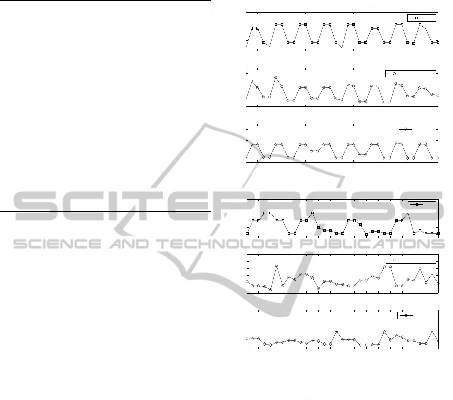
runs of the examined algorithms. Periodical fluctu-
ations of best individuals that are visible on the plots
relate to rapid reactivity to the environmental changes
in G24 1 whereas the distorted irregular variations in-
dicate losing track of global optima. On the other
hand, mFDA1 is designed in such manner that the
ideal run would result in the straight line at the 0 level.
Thus, each deviation towards positive values visible
on the plots signifies slow reaction to the environmen-
tal changes. Note that IDEA with restart hardly ap-
proached the 0 level. This implies that global optima
in mFDA1 are evidently less accessible by purely ran-
dom individuals then in G24 1. However, an antici-
pation mechanism of IDEA-FPS allowed for handling
with these difficulties.
In the experiments, the fixed sizes of the three
fractions were used which required some prior ex-
amination of the optimized problems. For practical
applications it would be more convenient to utilize a
self-adaptation mechanism responsible for selecting
the proper sizes. The future work should address that
issue at first.
5.3 Anticipation of Landscape Changes
This anticipation strategy is based on a Markov chain
model — a tool that is frequently applied in statis-
tics and data analysis. In the most general form a
Markov chain can be formulated as a sequence of ran-
dom variables (X
n
)
n∈N
, i.e. X
1
,X
2
,X
3
,.. ., such that
for all n ∈ N
P(X
n+1
= x |X
n
= x
n
,.. . ,X
1
= x
1
) =
= P(X
n+1
= x |X
n
= x
n
).
(5)
It means that the instance of X
n+1
depends only on its
predecessor X
n
, regardless the remaining of the his-
tory trail.
A discrete chain Markov model can be defined as
a tuple (S,T,λ), where S = {S
1
,S
2
,.. . ,S
m
} ⊂ R
d
(for
d ≥ 1) is a finite set of possible states (i.e. a do-
main of X
n
), T = [t
i j
] is a transition matrix contain-
ing probabilities of switching from state S
i
to S
j
(for
1 ≤ i, j ≤ m), and λ = (λ
1
,λ
2
,.. . ,λ
m
) is the initial
probability distribution of all the states in S.
Starting from the prior knowledge, which in
practice is often a zero knowledge, where λ =
(1/m,1/m,.. .,1/m), and by assuming that the vari-
ables X
n
are sampled from some unknown stochastic
process, the characterization of this process is built
iteratively by observing instances of X
n
and maintain-
ing the transition matrix T as follows. Let C = [c
i j
]
be an intermediary matrix for counting the past tran-
sitions. For all 1 ≤ i, j ≤ m the coefficients c
i j
hold
the number of transitions from state S
i
to S
j
that oc-
curred so far. After each such transition the value
of c
i j
is incremented. The matrix T is then built up
with the row-vectors T
i
= [c
i1
/c,c
i2
/c,.. . ,c
im
/c] for
i = 1,.. . ,m, where c =
∑
m
j=1
c
i j
.
The assumption stated in Equation 5 implies that
any row T
i
of matrix T indeed estimate the probabil-
ity distribution of switching from the state S
i
to any
of the possible states S
j
∈ S. As a consequence, the
model of changes encoded in T can be used further for
predicting the future value of X
n
for at least one step
ahead by simply picking up the most probable transi-
tion originating at the present state. This mechanism
is typically referred to as a Markov chain predictor.
The fundamental aspect in applying a Markov
chain predictor is the definition of S. Ideally, the states
S
1
,S
2
,.. . ,S
m
should play the role of snapshots, i.e.
the exact models of the landscape at the given time.
However, when dealing with optimization problems
the main impact is on localizing the optimum, thus
the quality of the model for the remaining part of the
search space is negligible.
In (Sim
˜
oes and Costa, 2013), the authors applied
a Markov chain predictor to the EA in order to im-
prove its rapidness in solving the bit-string problems
with the recurring type of changes. In this approach
the applicability of the above mechanism is extended
to the continuous domain. Note that, unlike bit-string
problems where identifying the states of the environ-
ment is rather straightforward, in the case of continu-
ous domain some parametrization is required for stor-
ing information about the landscape. For this pur-
pose, a stochastic parametrization utilized in Estima-
tion of Distribution Algorithms (EDAs) (Larra
˜
naga
and Lozano, 2001) seems most adequate since it mod-
els the exact spatial locations of the best candidate so-
lutions.
IJCCI2014-DoctoralConsortium
8

EDAs are the class of EAs that search for the op-
tima by building up a probabilistic model of the most
promising regions in the vector space. They typically
begin with a zero knowledge or a very rough estima-
tion concerning the expected location of the optimum.
Later on, the more exact model of the landscape is ac-
quired iteratively by performing a random sampling
in the area of interest and then narrowing down this
area by cutting off the regions containing “the worst
samples”. Then, sampling it again and so on until
convergence.
Univariate Marginal Distribution Algorithm
(UMDA) (Liu et al., 2008) falls under the umbrella
of EDAs. It estimates the distribution of the best
individuals in the d-dimensional search space (d > 1)
however the mutual independence of all d coefficients
is assumed in order to simplify the computation.
In the proposed approach, the states of the en-
vironment are characterized with Gaussian distribu-
tions that model the spatial locations of best candi-
date solutions in the search space. For all i = 1,... ,m
holds S
i
≡ (µ
i
,Σ
i
) where µ
i
∈ R
d
is a mean vector and
Σ
i
= [σ
kl
]
1≤k,l≤d
is a covariance matrix. These param-
eters are estimated and delivered by UMDA. Later on,
the outputs of a Markov chain predictor are utilized by
the same UMDA to direct the optimization towards
the future promising regions.
The modification of UMDA equipped with the an-
ticipation mechanism was named UMDA-MI
1
(Filip-
iak and Lipinski, 2014b). Similarly to IDEA-FPS, it
maintains the three fractions of candidate solutions —
exploring, exploiting and anticipating. Like before,
the first one is filled up with random immigrants sam-
pled with the uniform distribution across the search
space. The remaining two fractions are formed with
the individuals sampled as follows. Let Φ and
e
Φ be
Gaussian distributions. The exploiting fraction uses
the present distribution model Φ that is updated itera-
tively during the run of UMDA-MI whereas the antic-
ipating fraction uses the foreseen distribution model
e
Φ obtained from the Markov chain predictor.
Algorithm 3 presents the main loop of UMDA-
MI. It begins with a random selection of the distribu-
tion Φ
1
= (µ
1
,Σ
1
) and defining the empty chain pre-
dictor (S, T, λ) = (
/
0,[],1). The anticipated distribu-
tion
e
Φ
1
is set to Φ
1
as for UMDA-MI it is established
that in case of no clear forecast about the next envi-
ronmental change, the best prediction available is in
fact the present distribution Φ
t
.
The algorithm runs for N
gen
> 0 generations, each
of which is split into N
sub
> 0 intermediary steps
called subiterations. Every k-th subiteration (for k =
1
The letter ’M’ stands for a Markov chain predictor
while ’I’ for random immigrants.
1,.. . ,N
sub
) includes generating the three fractions of
candidate solutions as follows. The exploring fraction
is filled with size
explore
random individuals, while the
exploiting and anticipating fractions are formed with
size
exploit
and size
anticip
candidate solutions sampled
with the distribution models Φ
t
k
and
e
Φ
t
k
respectively.
Next, all the fractions are grouped together and evalu-
ated. Among them the top 0 < M
best
< M individuals
p
1
, p
2
,.. . , p
M
best
∈ R
d
are filtered out and utilized for
updating the estimation of distribution Φ
t
k
= (µ
t
k
,Σ
t
k
)
using the following formula
µ
t
k
=
M
best
∑
i=1
p
i
M
best
, σ
t
k
=
q
∑
M
best
i=1
(p
i
− µ
t
k
)
2
M
best
. (6)
At the beginning of each generation, UMDA-MI
sets all the fraction sizes to 1/3 and then updates them
automatically N
sub
times, i.e. once per subiteration.
The updating rule works as follows. It begins with
finding a single best individual per fraction as its rep-
resentative. Then, all the three fractions are given la-
bels adequate to the fitness of their respective repre-
sentatives. The fraction containing the best represen-
tative is labeled best, the second best is labeled
Algorithm 3: Pseudo-code of UMDA-MI.
Initialize estimation of distribution Φ
1
randomly
Initialize Markov Chain predictor by setting:
(S,T,λ) = (
/
0,[],1) and
e
Φ
1
= Φ
1
for t = 1 → N
gen
do
Φ
t
1
= Φ
t
size
explore
= size
exploit
= size
anticip
= 1/3
for k = 1 → N
sub
do
P
explore
= RandomImmigrants(size
explore
)
P
exploit
= GenerateFraction(Φ
t
k
,size
exploit
)
P
anticip
= GenerateFraction(
e
Φ
t
,size
anticip
)
P
t
k
= P
explore
∪ P
exploit
∪ P
anticip
Evaluate(P
t
k
)
UpdateEstimation(Φ
t
k
,P
t
k
)
UpdateFractionSizes(P
explore
,P
exploit
,P
anticip
)
end for
S = S ∪ {Φ
t
k
}
if size(S) = max-size(S) then
Find a pair {S
i
,S
j
} of the most similar states
in the set S
S
i j
= AverageState({S
i
,S
j
})
Replace {S
i
,S
j
} with S
i j
in the set S
end if
Update transition matrix T
Assign Φ
t+1
to the most similar state to Φ
t
k
in the set S
e
Φ
t+1
= PredictNextState(Φ
t+1
)
end for
ProactiveEvolutionaryAlgorithmsforDynamicOptimizationProblems
9

Table 2: The best-of-generation results averaged over 50 independent runs for the compositions of Sphere, Rastrigin,
Griewank and Ackley functions.
Dimensions 5 10
Function N
sub
2 5 10 20 2 5 10 20
SGA-R 216.0 149.7 90.4 59.7 441.0 350.2 246.5 129.0
Sphere UMDA 129.6 92.8 78.1 71.5 151.5 107.7 89.2 77.5
UMDA-MI 94.4 62.1 57.7 56.5 109.8 77.4 62.2 59.0
SGA-R 586.3 438.1 350.0 312.1 845.6 717.1 621.4 585.8
Rastrigin UMDA 560.3 429.6 438.8 354.8 713.1 608.6 533.9 462.0
UMDA-MI 370.9 312.1 263.7 229.5 532.9 488.0 441.7 409.2
SGA-R 350.9 272.7 202.3 159.9 522.8 437.7 335.7 224.3
Griewank UMDA 224.5 188.4 153.5 132.2 234.6 201.7 176.7 158.2
UMDA-MI 203.9 160.7 129.9 113.2 205.4 172.0 148.9 140.2
SGA-R 1687.4 1508.6 1176.4 665.5 1886.9 1831.2 1740.7 1507.2
Ackley UMDA 1657.3 1613.6 1476.2 1364.6 1597.2 1587.4 1441.6 1343.2
UMDA-MI 965.9 742.3 485.6 403.9 1093.4 858.9 645.7 516.0
medium and the last one — worst. Next, the size
of the best fraction is increased by the small con-
stant ε > 0. The remaining 1 − size
best
“vacant slots”
are disposed between the medium and worst fractions
proportionally to the differences in fitness of their rep-
resentatives and the representative of the best fraction.
Clearly, all the three sizes must sum up to 1. They
are also restricted to the range [size
min
,size
max
] where
0 < size
min
< size
max
< 1 in order to prevent from the
excessive domination of a certain fraction causing the
exclusion of the others.
After completing all of the N
sub
subiterations, the
Markov chain predictor is launched (once per gener-
ation). Firstly, it adds the obtained distribution Φ
t
k
to
the set of possible states S. Later, if the number of
elements of S (after extending) reaches the predefined
maximum size, the following replacement procedure
is executed. Among all the elements in S a single pair
of the two most similar states {S
i
,S
j
} ⊂ S is identified
and replaced with their average S
i j
. In order to find
the most similar state to S
i
, for all i = 1, ... , size(S) a
number of random samples is generated according to
S
i
and compared with S \ {S
i
}. A Gaussian with the
highest response to these samples is selected as S
j
. In
the case when S
i
or S
j
is the present state of environ-
ment, the state S
i j
takes over its role.
The transition matrix T is built and maintained us-
ing the intermediary counting matrix C as described
before. However, each time the two states S
i
and S
j
are unified, the corresponding j-th row and j-th col-
umn of C are removed while their values are added to
the respective elements of i-th row and i-th column.
Finally, the most probable future state according
to T is picked and used as the distribution model for
the next anticipating fraction
e
Φ
t+1
.
UMDA-MI was tested on the DOPs generated
with the Dynamic Composition Benchmark Gener-
ator (DCBG) (Li et al., 2008) which rotates and
aggregates the functions given as input in a time-
dependent manner. In the experiments the com-
ponents of Sphere, Rastrigin, Griewank and Ackley
functions were used.
Table 2 summarizes the best-of-generation results
(i.e. mean evaluations of the best solutions found
just before the next environmental change) averaged
over 50 independent runs with various problem di-
mensions d ∈ {5, 10} and numbers of subiterations
N
sub
∈ {2,5,10,20}. For comparison, also a Simple
Genetic Algorithm with a complete re-initialization
of a population after each change of the landscape
(SGA-R) was run. It is evident that UMDA-MI out-
performed both UMDA and SGA-R in all the exam-
ined cases.
The preliminary experiments revealed that the ap-
plication of a Markov chain predictor together with
the introduction of random immigrants into UMDA
significantly improved the algorithm’s reactivity to
the recurrently changing environments in the contin-
uous domain. However, it is probable that the ac-
curacy of a Markov chain predictor may deteriorate
in other than recurrent types of changes. The future
work should cover that as well as dealing with the
presence of constraints.
5.4 Time-linkage Aspect
The time-linkage aspect is an issue raised in (Bosman,
2005; Nguyen and Yao, 2009b). It assumes that any
decision made at the given moment t ∈ T may in-
fluence the states of the environment in the future.
This implies that a solution which seemed optimal in
the short-time perspective can unexpectedly become a
IJCCI2014-DoctoralConsortium
10

sub-optimal one when perceived on the long term ba-
sis. For instance, a buy/sell decision of large amounts
of assets on the stock market might affect the other
players and result in a significant change of the prices.
The above aspect in DOPs is still not well stud-
ied. Moreover, it appears an extremely difficult issue
to tackle in the proactive model since it requires the
highly-accurate long-term forecasts.
It is very tempting to modify the three anticipation
strategies presented in the previous sections such that
they could try to deal with the time-linkage. How-
ever, this requires a slight redefinition of the solution
to DOP. It should no longer be seen as the trajectory of
moving optima, yet rather a more abstract entity like a
consistent strategy or a classificator suggesting the be-
haviour in given states of the environment which can
be further evaluated from the long-term perspective.
6 EXPECTED OUTCOME
The proposed anticipation strategies ought to be veri-
fied in the large set of both benchmark and real-world
DOPs. It is expected that, after a thorough examina-
tion, the groups of problems that can be handled well
with these strategies will be clearly identified.
It is also believed that at least some examples of
the time-linkage can also be dealt with using the sug-
gested anticipation strategies or their modifications.
Finally, one can expect that a comparison with
other proactive approaches will result in some fu-
ture improvements of IDEA-ARIMA, IDEA-FPS and
UMDA-MI including an addition of auto-adaptation
mechanisms, a reduction of the number of input pa-
rameters or an application of other prediction models.
REFERENCES
Bosman, P. A. N. (2005). Learning, anticipation and time-
deception in evolutionary online dynamic optimiza-
tion. In Proceedings of the 2005 workshops on Ge-
netic and evolutionary computation, pages 39–47.
Box, G. E., Jenkins, G. M., and Reinsel, G. C. (2011). Time
series analysis: forecasting and control, volume 734.
John Wiley & Sons.
Branke, J. (2001). Evolutionary optimization in dynamic
environments. Kluwer Academic Publishers.
Brzychczy, E., Lipinski, P., Zimroz, R., and Filipiak, P.
(2014). Artificial immune systems for data classifi-
cation in planetary gearboxes condition monitoring.
In Advances in Condition Monitoring of Machinery in
Non-Stationary Operations, LNME, pages 235–247.
Springer.
Castellani, M. and Fahmy, A. A. (2008). Learning the in-
verse kinematics of a robot manipulator using the bees
algorithm. In Proceedings of the 6th IEEE Interna-
tional Conference on Industrial Informatics (INDIN
2008), pages 493–498.
Cobb, H. G. (1990). An investigation into the use of hyper-
mutation as an adaptive operator in genetic algorithms
having continuous, time-dependent nonstationary en-
vironments. Technical Report AIC-90-001.
Deb, K., Pratap, A., Agarwal, A., and Meyarivan, T. (2002).
A fast and elitist multiobjective genetic algorithm:
NSGA-II. IEEE Transactions on Evolutionary Com-
putation, 6:182–197.
Eggermont, J., Lenaerts, T., Poyhonen, S., and Termier, A.
(2001). Raising the dead: Extending evolutionary al-
gorithms with a case-based memory. Genetic Pro-
gramming, pages 280–290.
Farina, M., Deb, K., and Amato, P. (2004). Multiobjec-
tive optimization problems: Test cases, approxima-
tions and applications. IEEE Transactions on Evolu-
tionary Computation, 8(5):425–442.
Filipiak, P. and Lipinski, P. (2012). Parallel CHC algo-
rithm for solving dynamic traveling salesman problem
using many-core GPU. In Proceedings of Artificial
Intelligence: Methodology, Systems and Applications
(AIMSA 2012), volume 7557 of LNAI, pages 305–314.
Springer.
Filipiak, P. and Lipinski, P. (2014a). Infeasibility driven
evolutionary algorithm with feed-forward prediction
strategy for dynamic constrained optimization prob-
lems. In EvoApplications 2014, LNCS. Springer.
Filipiak, P. and Lipinski, P. (2014b). Univariate marginal
distribution algorithm with markov chain predictor in
continuous dynamic environments. In Proceedings of
Intelligent Data Engineering and Automated Learning
(IDEAL 2014), LNCS. Springer.
Filipiak, P., Michalak, K., and Lipinski, P. (2011). Infea-
sibility driven evolutionary algorithm with ARIMA-
based prediction mechanism. In Proceedings of In-
telligent Data Engineering and Automated Learning
(IDEAL 2011), volume 6936 of LNCS, pages 345–
352. Springer.
Filipiak, P., Michalak, K., and Lipinski, P. (2012a).
Evolutionary approach to multiobjective optimiza-
tion of portfolios that reflect the behaviour of in-
vestment funds. In Proceedings of Artificial In-
telligence: Methodology, Systems and Applications
(AIMSA 2012), volume 7557 of LNAI, pages 202–211.
Springer.
Filipiak, P., Michalak, K., and Lipinski, P. (2012b). A
predictive evolutionary algorithm for dynamic con-
strained inverse kinematics problems. In Proceedings
of Hybrid Artificial Intelligence Systems (HAIS 2012),
volume 7208 of LNCS, pages 610–621. Springer.
Grefenstette, J. (1992). Genetic algorithms for changing en-
vironments. In Parallel Problem Solving from Nature
2, pages 137–144.
Hatzakis, I. and Wallace, D. (2006). Dynamic multi-
objective optimization with evolutionary algorithms:
A forward-looking approach. In Proceedings of the
ProactiveEvolutionaryAlgorithmsforDynamicOptimizationProblems
11

8th annual conference on Genetic and evolutionary
computation (GECCO 2006), pages 1201–1208.
Jozefowiez, N., Semet, F., and Talbi, E.-G. (2009). An
evolutionary algorithm for the vehicle routing prob-
lem with route balancing. European Journal of Oper-
ational Research, 195(3):761–769.
Kim, K. (2006). Artificial neural networks with evolution-
ary instance selection for financial forecasting. Expert
Systems with Applications, 30(3):519–526.
Lancucki, A., Chorowski, J., Michalak, K., Filipiak, P., and
Lipinski, P. (2014). Continuous population-based in-
cremental learning with mixture probability modeling
for dynamic optimization problems. In Proceedings of
Intelligent Data Engineering and Automated Learning
(IDEAL 2014), LNCS. Springer.
Larra
˜
naga, P. and Lozano, J. A. (2001). Estimation of Dis-
tribution Algorithms: A New Tool for Evolutionary
Computation. Kluwer Academic Publishers.
Li, C., Yang, S., Nguyen, T. T., Yu, E. L., Yao, X., Jin, Y.,
Beyer, H.-G., and Suganthan, P. N. (2008). Bench-
mark generator for cec 2009 competition on dynamic
optimization. Technical report, University of Leices-
ter, University of Birmingham, Nanyang Technologi-
cal University.
Liu, X., Wu, Y., and Ye, J. (2008). An improved estimation
of distribution algorithm in dynamic environments. In
Proceedings of the IEEE Fourth International Confer-
ence on Natural Computation (ICNC 2008), volume 6,
pages 269–272.
Michalak, K., Filipiak, P., and Lipinski, P. (2013). Usage
patterns of trading rules in stock market trading strate-
gies optimized with evolutionary methods. In EvoAp-
plications 2013, volume 7835 of LNCS, pages 234–
243. Springer.
Michalak, K., Filipiak, P., and Lipinski, P. (2014). Multi-
objective dynamic constrained evolutionary algorithm
for control of a multi-segment articulated manipulator.
In Proceedings of Intelligent Data Engineering and
Automated Learning (IDEAL 2014), LNCS. Springer.
Nguyen, T. T. and Yao, X. (2009a). Benchmarking and solv-
ing dynamic constrained problems. In Proceedings
of the IEEE Congress on Evolutionary Computation
(CEC 2009), pages 690–697.
Nguyen, T. T. and Yao, X. (2009b). Dynamic time-
linkage problems revisited. Applications of Evolution-
ary Computing, pages 735–744.
Richter, H. and Yang, S. (2008). Memory based on ab-
straction for dynamic fitness functions. In EvoWork-
shops 2008, volume 4974 of LNCS, pages 596–605.
Springer.
Rossi, C., Abderrahim, M., and D
´
ıaz, J. C. (2008). Track-
ing moving optima using Kalman-based predictions.
Evolutionary Computation, 16(1):1–30.
Sim
˜
oes, A. and Costa, E. (2011). CHC-based algorithms for
the dynamic traveling salesman problem. In Appli-
cations of Evolutionary Computation, volume 6624,
pages 354–363.
Sim
˜
oes, A. and Costa, E. (2013). Prediction in evolutionary
algorithms for dynamic environments. Soft Comput-
ing, pages 1–27.
Singh, H. K., Isaacs, A., Nguyen, T. T., Ray, T., and Yao,
X. (2009a). Performance of infeasibility driven evolu-
tionary algorithm (IDEA) on constrained dynamic sin-
gle objective optimization problems. In Proceedings
of the IEEE Congress on Evolutionary Computation
(CEC 2009), pages 3127–3134.
Singh, H. K., Isaacs, A., Ray, T., and Smith, W. (2009b).
Infeasibility driven evolutionary algorithm for con-
strained optimization. Constraint Handling in Evo-
lutionary Optimization, Studies in Computational In-
telligence, pages 145–165.
van Hemert, J., van Hoyweghen, C., Lukschandl, E., and
Verbeeck, K. (2001). A “futurist” approach to dy-
namic environments. In GECCO EvoDOP Workshop,
pages 35–38.
Vavak, F., Jukes, K., and Fogarty, T. C. (1997). Adap-
tive combustion balancing in multiple burner bolier
using a genetic algorithm with variable range of local
search. In Proceedings of the International Confer-
ence on Genetic Algorithms (ICGA 1997), pages 719–
726.
Yang, S. (2005). Memory-based immigrants for genetic al-
gorithms in dynamic environments. In Proceedings
of the IEEE Congress on Evolutionary Computation
(CEC 2005), pages 1115–1122.
Yang, S. (2006). On the design of diploid genetic algorithms
for problem optimization in dynamic environments.
In Proceedings of the IEEE Congress on Evolutionary
Computation (CEC 2006), pages 1362–1369.
Yang, S. and Yao, X. (2008). Population-based incremental
learning with associative memory for dynamic envi-
ronments. IEEE Transactions on Evolutionary Com-
putation, 12(5):542–561.
Zhou, A., Jin, Y., Zhang, Q., Sendhoff, B., and Tsang, E.
(2007). Prediction-based population re-initialization
for evolutionary dynamic multi-objective optimiza-
tion. Evolutionary Multi-Criterion Optimization,
pages 832–846.
APPENDIX
Infeasibility Driven Evolutionary
Algorithm
Infeasibility Driven Evolutionary Algorithm (IDEA)
(Singh et al., 2009b) was originally proposed to ad-
dress stationary constrained optimization problems. It
maintains a certain fraction of “good” yet infeasible
solutions within a population in order to improve an
exploration of areas near constraint boundaries.
IDEA evaluates each individual under the two cri-
teria. One criterion is simply an objective function.
Another criterion, called violation measure, deter-
mines to what extent a given solution violates the con-
straints.
IJCCI2014-DoctoralConsortium
12

Algorithm 4: IDEA-Reduction of a union C ∪ P of children
and parents populations respectively, producing an output
population P
0
of M > 0 individuals.
M
in f eas
= size
in f eas
· M
M
f eas
= M − M
in f eas
(S
f eas
,S
in f eas
) = Split(C ∪ P)
Rank(S
f eas
)
Rank(S
in f eas
)
P
0
= S
f eas
(1 : M
f eas
) + S
in f eas
(1 : M
in f eas
)
Algorithm 5: Sub-IDEA step.
P
1
= P
Evaluation(P
1
)
for t = 1 → N
sub
do
P
0
t
= Selection(P
t
)
C
t
= Crossover(P
0
t
)
C
00
t
= Mutation(C
0
t
)
P
t+1
= IDEA-Reduction(P
t
∪C
00
t
)
end for
Return P
N
sub
Algorithm 6: Main loop of IDEA.
P
1
= RandomPopulation()
for t = 1 → N
gen
do
Evaluation(P
t
)
C
t
= Sub-IDEA(P
0
t
)
P
00
t
= IDEA-Reduction(P
0
t
∪C
t
)
end for
Since IDEA essentially reformulates a single-
objective problem into a multi-objective one, any
two individuals can no longer be compared accord-
ing to their fitness. Instead, the ranking based on
non-dominated sorting procedure with crowding dis-
tance metric (as a tie-breaking rule) is performed as
in NSGA-II (Deb et al., 2002). It is important to note
that crowding distance promotes individuals located
in less crowded areas hence it introduces diversity
within a population.
One of the key aspects of IDEA is the specific im-
plementation of a reduction step. As it is seen in Al-
gorithm 4, individuals from C ∪ P (a union of chil-
dren and parents populations) are firstly split into two
subsets containing feasible and infeasible solutions —
S
f eas
and S
in f eas
respectively. Then, both subsets are
ranked according to the mentioned NSGA-II ranking.
Afterwards, the top M
f eas
individuals of S
f eas
and the
top M
in f eas
individuals of S
in f eas
are chosen to form
the new generation P
0
. Such separation is intended
to promote the infeasible individuals which otherwise
could be eliminated by the feasible ones due to their
superiority in violation measure.
From the implementation perspective the heart of
IDEA is Sub-IDEA step (Algorithm 5) which essen-
tially runs the entire “evolutionary engine” of the al-
gorithm. It consists of N
sub
> 0 iterations of tourna-
ment selection, simulated binary crossover (SBX) and
polynomial mutation (Singh et al., 2009b). In order
not to confuse iterations of Sub-IDEA step with itera-
tions of the main loop, the former ones are referred to
as subiterations.
The main loop of IDEA (presented in Algo-
rithm 6), apart from invoking Sub-IDEA step, con-
sists only of one re-evaluation of a population and one
IDEA-Reduction step per iteration.
ProactiveEvolutionaryAlgorithmsforDynamicOptimizationProblems
13
