
STDP Learning Under Variable Noise Levels
Dalius Krunglevicius
Faculty of Mathematics and Informatics, Vilnius University, Naugarduko st 24, Vilnius, Lithuania
Keywords: Artificial Neural Networks, Spike-Timing-Dependent Plasticity, STDP, Hebbian Learning, Unsupervised
Learning, Temporal Coding, Neuroscience.
Abstract: Spike-timing-dependent plasticity (STDP) is a set of Hebbian learning rules which are firmly based on
biological evidence. It has been demonstrated that one of the STDP learning rules is suited for learning
spatiotemporal patterns in a very noisy environment. Parameters of the neuron are only optimal, however,
for a certain range of quantity of injected noise. This means the level of noise must be known beforehand so
that the parameters can be set accordingly. That could be a real problem when noise levels vary over time.
We found that the model of a leaky-integrate-and-fire inhibitory neuron with an inverted STDP learning rule
is capable of adjusting its response rate to a particular level of noise. In this paper we suggest a method that
uses an inverted SDTP learning rule to modulate spiking rate of the trained neuron. This method is adaptive
to noise levels; subsequently spiking neuron can be trained to learn the same spatiotemporal pattern with a
wide range of background noise injected during the learning process.
1 INTRODUCTION
Spiking neural networks (SNNs) are third generation
artificial neural networks (Maas, 1997). Compared
to previous generations, SNNs are more biologically
based than their predecessors. Because of large
computational costs, the applications of SNNs in
machine learning or pattern recognition is
problematic for the moment. It is reasonable to
expect, however, that growing computer power will
make SNNs practical in the near future. The main
motivation behind this paper is research on how
SNNs can be applied to pattern recognition in
particular. In this paper we address the problems
associated with training SNNs for spatiotemporal
pattern recognition.
Neurons of most animal species communicate by
releasing chemical messengers called
neurotransmitters during an atomic event called a
spike. There are two major approaches to interpret
neural spikes as data. One is rate coding, where data
are encoded in an averaged count of spikes over a
specific time window. The other is temporal coding,
where data are encoded within the precise timing of
an individual spike.
In this paper we address temporal coding only.
Findings from biological research suggest that
rate coding alone cannot account for the speed of
data transfer in living organisms (Gerstner et al.,
1996; VanRullen and Thorpe, 2001). Temporal
coding, on the other hand, can, because it requires
very minimal time for the neuron to respond. It is
debatable if temporal coding does take place in
living neural systems (Rolls et al., 2004), however
there is experimental evidence to support the
concept of temporal coding (Gerstner and Kistler,
2002; Fellous et al., 2004; VanRullen et al., 2005,
Kayser et al., 2009). Moreover, the discovery of
spike-timing-dependent plasticity (STDP) suggests
that the timing of the spikes is what matters. STDP
is a function of time difference between presynaptic
and postsynaptic spikes that guards the amount of
change of synaptic strength. Persistent increases of
synaptic strength are referred as long-term
potentiation (LTP), while persistent decreases are
referred as long-term depression (LTD). There are a
few distinct STDP rules of different types of
synapses known at the moment (Caporale and Dan,
2008). STDP is often referred to as a form of
Hebbian learning.
One of the possible interpretations of temporal
coding is as a spatiotemporal pattern. The simplest
example of a spatiotemporal pattern is a binary
on/off map of spikes in a short temporal window,
where the probability of the spike at the “on”
synapse is significantly larger than at the “off”
synapses and “on” spikes are largely correlated in
165
Krunglevicius D..
STDP Learning Under Variable Noise Levels.
DOI: 10.5220/0005072401650171
In Proceedings of the International Conference on Neural Computation Theory and Applications (NCTA-2014), pages 165-171
ISBN: 978-989-758-054-3
Copyright
c
2014 SCITEPRESS (Science and Technology Publications, Lda.)

time, while “off” spikes are not and produce only
noise. In the case of STDP learning, under a certain
range of parameters, the strengths of the synapses
associated with the pattern grow, while the strengths
of other synapses which receive only noise decay. In
other words, the individual neuron acts as
coincidence detector (Abbott and Nelson, 2000). In
the simplest case possible, when the pattern is static
and background noise is absent, such training can be
reduced to supervised learning as a simple
assignment operation: set strength to 1 if input is in
the pattern, set to 0 otherwise.
Figure 1: STDP training rules addressed in this paper. w
is the amount of change in synaptic strength; t is time
difference between postsynaptic and presynaptic spikes. a)
STDP rule of excitatory-to-excitatory synapses. b) STDP
rule of excitatory-to-inhibitory synapses. c) Update is
guarded by the nearest–neighbour rule with immediate
pairings only (Burkitt et al. 2004: Model IV).
The STDP rule of excitatory-to-excitatory
synapses (Figure 1a) is the most widely researched
one. In this paper we will refer to this rule as STDP
rule A. When using this rule, and organizing
multiple neurons in a competitive network, that is,
connecting neurons with lateral inhibitory synapses,
it is possible to train that network for multiple
distinct spatiotemporal patterns, where individual
neuron becomes selective for only one of the
patterns. This has been demonstrated by many
authors (Masquelier et al., 2009; Song et al., 2000;
Guyonneau et al., 2005; Gerstner and Kistler, 2002).
Such a network is capable of learning even if the
pattern is highly obscured by noise (Masquelier et
al., 2008, 2009). SDTP learning of spatiotemporal
patterns holds potential for practical pattern
recognition, something explored by other authors
(Gupta and Long , 2007; Nessler et al., 2009; Hu et
al., 2013; Kasabov et al., 2013).
In this paper we address the problem associated
with levels of noise injected during the training of a
neuron. Values of the neuron threshold, amplitude of
relative refraction and initial synaptic strengths
might be optimal only for a certain range of amounts
of injected noise. These parameters define the initial
spiking rate of the neuron (See Methods and
Parameters for further details). This means the level
of noise must be known beforehand, so the
parameters can be set accordingly. It could be a real
problem if the level of noise changes over time. To
overcome this problem, we introduced inhibitory
neurons which received excitatory input from the
same neurons as the training neuron. We used an
inverted STDP rule for excitatory-to-inhibitory
synapses (Figure 1b). In this paper we refer to this
rule as STDP rule B.
A similar rule of excitatory-to-inhibitory
synapses has been discovered in a cerebellum-like
structure of an electric fish (Bell et al., 1997) and in
mice (Tzounopoulos et al. 2004, 2007). The rule in
Figure 1b is not precisely the same: in the electric
fish LTD gradually becomes LTP, while in mice
there was zero LTP.
We found the model of an inhibitory neuron with
the inverted STDP learning rule is capable of
adjusting its response rate to a particular level of
noise. In this paper we suggest a method that uses an
inverted SDTP learning rule to modulate spiking rate
of the trained neuron. This method is adaptive to
noise levels; subsequently spiking neuron can be
trained to learn the same spatiotemporal pattern with
a wide range of background noise injected during
the learning process.
2 SOME PROPERTIES OF THE
INVERTED STDP RULE
2.1 Training for Poisson Noise
We exposed neurons with the different threshold
values to Poisson noise. Each trained neuron
received input from 4,096 input neurons which
produced Poisson noise by producing an input spike
with a probability of 0.02 at each discrete step in the
simulation. STDP rules A and B were compared.
Results are represented in Figure 2. See Methods
and Parameters for further details.
When exposed to Poisson noise only, STDP rule
A, as expected, leads to two possible outcomes:
either synaptic strengths decay until the neuron is
not capable of firing, or all synaptic strengths grow
and the neuron is activated by any random spike
from the input.
The behavior of inverted rule B is far more
NCTA2014-InternationalConferenceonNeuralComputationTheoryandApplications
166
interesting: the neuron tends to stabilize its firing
rate at a certain point. The point of stable firing rate
depends on more than just threshold variables and
the level of noise: the training step and initial values
of synaptic strengths are very important as well. It
seems that in case of rule B capping of synaptic
strengths to some maximal value is not required.
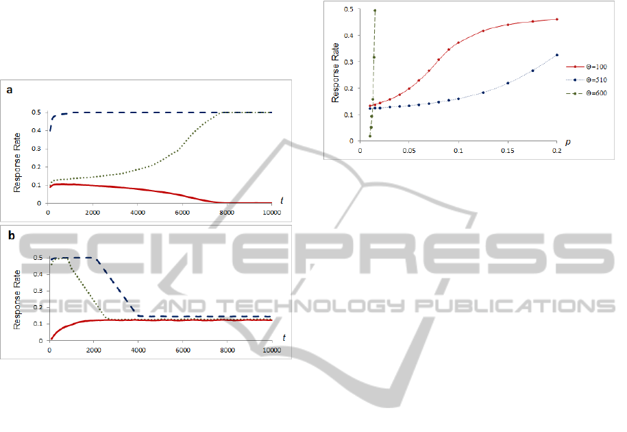
Figure 2: Comparison of STDP rules A and B, response
rates to the same level of Poisson noise and different
neuron thresholds. Vertical axis represents the response
rate; horizontal axis represents the simulation time. a)
STDP rule A, dashed line denotes a threshold value
=100, dotted line =340, solid line =900. b) STDP
rule B, dashed line at threshold value =100, dotted line
=160, solid line =170.
In this case, if noise is mixed with a recurring
spatiotemporal pattern of sufficient size, STDP rule
B also leads to remembering the pattern in synaptic
strengths, but in an inverted manner: synapses which
are associated to the pattern are weaker than those
not associated. When compared with rule A, the
variance of synaptic strengths after training is
significantly larger.
2.2 Stability of Response Rate at
Different Noise Levels
To illustrate the dependency of stable rate points on
the noise level of STDP rule B, we repeated the
experiment described in the previous section over a
range of Poisson noise. The results are presented in
Figure 3.
While noise levels increase, depending on a
neuron threshold value, firing rate slowly
approaches the maximum value, which is 0.5, since
the neuron has a period of absolute refraction equal
to one step of the simulation in our model.
Figure 3: Points of stability in STDP rule B. Vertical axis
represents the spiking rate; horizontal axis represents the
probability of a spike of an individual input neuron at each
discrete step of the simulation. Solid red line denotes a
threshold value =100; solid blue line =510; dashed
green line denotes response rates when synaptic strengths
are static, at =600.
The neuron with static synapses approaches
maximal response rate very rapidly in a narrow
range of stimulation (Figure 3, dashed green line).
Our goal was to get a neuron to provide inhibition in
proportion to the amount of background noise.
Therefore, we preferred STDP rule B instead of
static synapses.
3 METHODS AND PARAMETERS
3.1 Leaky Integrate-and-Fire Neuron
Neurons were modelled on a simplified version of
the Spike Response Model (SRM) (Gerstner and
Kistler, 2002). The original SRM model has a
smoothly decaying hyperpolarization function
during the refractory period, but has little or no
influence when the simulation time step and the
absolute refractory period combined are sufficiently
high to overstep the smooth curve, and this was the
case in our simulations. In the model potential P at
the time t of the neuron membrane is given by:
∆/
(1)
where W
r
and T
r
are the parameters that define the
amplitude and duration of relative refraction. Since
at the time of the spike the neuron is in the phase of
absolute refraction, the value of the membrane
potential plays no role in training. Therefore this
value is set to a constant just for ease of
visualization and convenience. The value of
STDPLearningUnderVariableNoiseLevels
167

postsynaptic potential coming in from an individual
synapse PSP(t) is given by:
∆
1
∆
1
(2)
where
t = t - t
pre
; w
j
is the strength of the synapse,
j
is the factor assigned to each individual synapse, it
can be 1 or -1 depending on synapse type; T
s
and T
m
are the time constants.
Variables
m
and
s
are given by:
∆
1
1
1
(3)
∆
1
1
1
(4)
Initial values of
m
and
s
are zero. Equations 3 and
4 were derived in the following way: the summed
values of individual PSPs of a single synapse at the
moment t can be expressed as a finite series:
⋯
(5)
where w
j
is the set of strengths at the moment of
each spike and t
j
is the set of times of spikes. The
expression is valid assuming that all t
j
<t. Treating
the positive and negative parts of the series
separately, the first two members of the series could
be expressed as the equation:
1
1
(6)
where
0
=0 at the beginning of the simulation.
Algebraically solving equation 6 gives the equations
3 and 4. Since in the discrete-time simulation,
exponentials functions can be pre-calculated, and
computed only at the time of the spike, this allows
minimizing computational costs.
Constants during the simulations were set to
values: T
m
=10; T
r
=10; T
s
=0.5; W
r
=2
; P
spike
=300.
is the neuron threshold value. The threshold value
of inhibitory neurons was fixed such that
inh
=1835.
3.2 Plasticity
The STDP window for excitatory-to-excitatory
synapses:
∆
⋅
∆
∆0
⋅
∆
∆0
0∆0
(7)
The STDP window for excitatory-to-inhibitory
synapses:
∆
⋅
∆
∆0
⋅
∆
∆0
0∆0
(8)
There
w
j
is a change in synaptic strength,
t is
time difference between presynaptic and
postsynaptic spikes, A
LTP
, A
LTD
, T
LTP
and T
LTD
are the
constants. Synaptic strengths were confined in
w
min
<w <w
max
.
Simulation constants for excitatory-to-excitatory
synapses were:
A
LTP
=0.75; A
LTD
=0.63; T
LTP
=16; T
LTD
=35;
w
min
=0.5; w
max
=30. Initial synaptic strengths were
uniformly distributed between 4.5 and 5.5.
Simulation constants for excitatory-to-inhibitory
synapses were:
A
LTP
=6.048; A
LTD
=7.2; T
LTP
=4; T
LTD
=16; w
min
=10
-
6
; w
max
=1.0. Initial synaptic strengths were
uniformly distributed between 0.9 and 1.0.
Synaptic strengths of static inhibitory synapses
was w=7.3 in the case of STDP rule B, and w=2.0
otherwise.
4 RESULTS
We measured the performance and success of the
training of a neuron for a spatiotemporal pattern.
The sample pattern was generated from 122 neurons
firing at the same time. The sample pattern was
demonstrated to the network periodically, in
intervals of 40 iterations. We executed the
experiment at a 1 ms scale, so that one iteration
corresponded to one millisecond. Overall there were
4,096 neurons in the input layer. All neurons in the
input layer produced noise except for the neurons
associated to the pattern at the moment of exposure
to the pattern (see Figure 6a).
The success of training was evaluated by
measuring differences between means of synaptic
strengths of synapses associated to the pattern and of
those which were not:
w
=
w_in
-
w_out
. Mean
values were scaled to range at the interval [0, 1]
respectively to the minimal and maximal values of
synaptic strengths. The criterion for successful
training was
w
> 0.85 at the end of the simulation.
Neurons which were unresponsive at the end of the
simulation were counted as unsuccessful, despite
possible large values for
w.
Performance of the
training was evaluated by measuring the velocity of
w
.
NCTA2014-InternationalConferenceonNeuralComputationTheoryandApplications
168
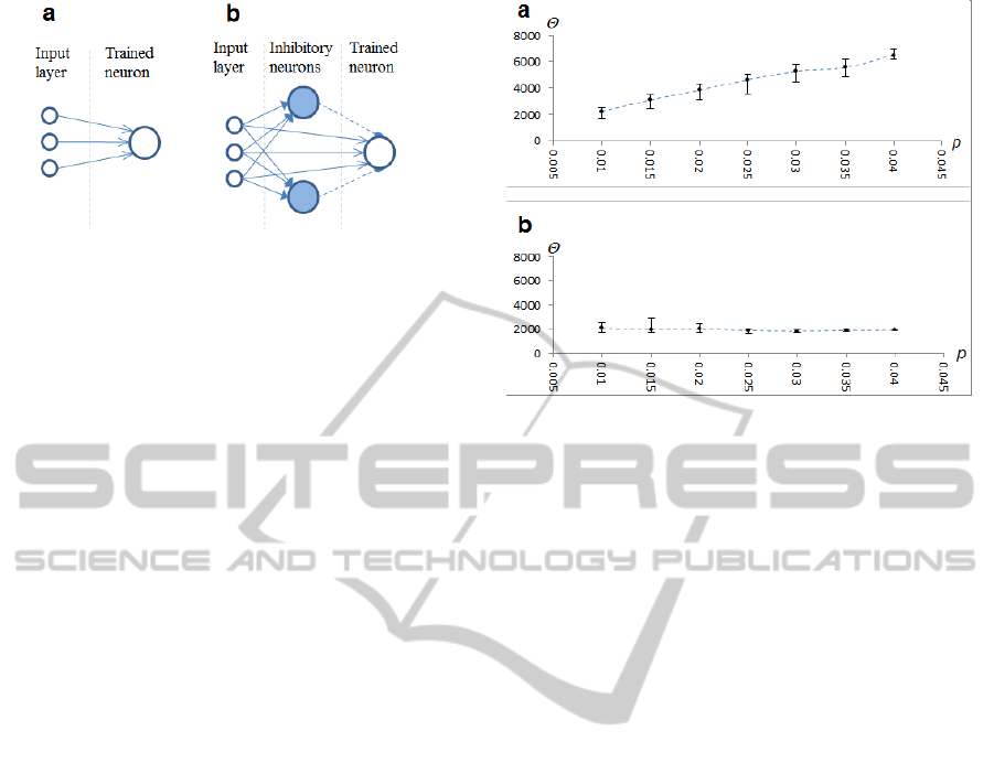
Figure 4: Neural network model. a) Simple network. b)
Network with vertical inhibition.
We compared the performance of a simple
neural network with that of a network with vertical
inhibition (Figure 4).
The neural network with vertical inhibition
consisted of an input layer, multiple inhibitory
neurons and the trained neuron. The trained neuron
received input from all neurons in the input layer,
while each inhibitory neuron received input from a
random fraction of an input layer (~10%). The
trained neuron had synapses with STDP rule A,
while inhibitory neurons had synapses with STDP
rule B. In addition the trained neuron received
inhibition from inhibitory neurons via static
synapses (Figure 4b).
In order to reduce variance in inhibitory
postsynaptic potentials (iPSP), we added multiple
inhibitory neurons instead of a single such neuron.
Variance of iPSPs reduces correlation between the
presynaptic spike of the sample pattern and the
postsynaptic spike; therefore, it has a negative
influence on the training process. By selecting only a
fraction of input neurons we ensured inhibitory
neurons would not fire synchronously. The network
contained 50 inhibitory neurons.
4.1 Training at Different Levels of
Constant Noise
We conducted a number of experiments at different
levels of Poisson noise mixed with a recurring
spatiotemporal pattern. Poisson noise was generated
by setting a fixed probability for an input spike at
each iteration of the simulation. Success of the
training was measured in a range of neuron
threshold values
. Amplitude of relative refraction
was set to W
r
=2
(see Methods and Parameters for
details).
In the case of a simple network (Figure 5a) we
observed, as expected, that under a fixed threshold
value, training is only possible within a narrow
range of noise levels.
Figure 5: Dependency of training success on neuron
threshold value and level of the injected Poisson noise.
Vertical axis represents the neuron threshold value
;
horizontal axis represents the level of noise. a) Results
from a simple network. Markers represent the point where
training was most rapid; error bars represent the range of
when training was successful. b) Results from a
network with vertical inhibition and STDP rule B.
In the case of the network with adaptive vertical
inhibition (Figure 5b), the optimal value for a
threshold was much less dependent on the level of
noise, and remained more or less stable. The same
neuron with a fixed threshold could be trained over
the broad range of noise levels we used in our
experiment (0.01 to 0.04). The range of possible
threshold values narrows, however, as noise
increases. This was due, most likely, to an increased
variance of postsynaptic potentials, which reduces
correlation between the spike from the input neuron
(presynaptic spike) and the spike of the trained
neuron (postsynaptic spike).
4.2 Training with Varying Noise Levels
In our next experiment we trained neurons with
variable levels of noise injected. We used a sine
function for setting the probability for the input
neuron to fire: p=0.01+0.015*((sin(t/
)+1)). See
Figure 6a. We evaluated training performance for
values 50, 100 and 150.
We compared the performance of a simple
network, the network with vertical inhibition and
STDP rule B, and a network with static synapses of
vertical inhibition. Results are presented in Figure
6b.
The training was executed over a range of a
neuron threshold values and only the best results
were taken into account.
STDPLearningUnderVariableNoiseLevels
169

Figure 6: Training with varying noise level. a) Example of
input spikes. Black dots represent fraction of a sample
pattern, grey dots represent injected noise. b) Values of
w
during the first 5,000 training iterations. Results are
from an experiment where =150. Solid red line denotes a
network with STDP rule B; dashed green line denotes a
network with static synapses of inhibitory neurons; dotted
blue line denotes a simple network.
In all cases of
, the network with STP rule B
performed best. The network with static inhibitory
neurons performed only slightly worse, which was a
somewhat surprising result. The simple network was
the worst performer because the trained neuron was
capable of firing only at peaks of stimulation from
the input layer.
5 DISCUSSION
We suggested a method that uses an inverted SDTP
learning rule to modulate spiking rate of the trained
neuron. We have shown that this method can be
applied to extend the range of noise levels under
which a neuron is able to learn a spatiotemporal
pattern. There are upper limits, however, for the
level of noise under which a neuron can be
successfully trained. By tuning the threshold value,
the neuron can be trained under conditions of much
more intense noise than we achieved in our
experiments. This is likely caused by the increased
variance introduced by vertical inhibition. This
problem requires additional research.
In our experiments we used a sample pattern of a
fixed size encoded as parallel singular spikes. This is
not a necessary condition: the sample pattern can be
encoded as parallel spike bursts or as parallel fixed
temporal patterns (Masquelier et al., 2008) and the
sample patterns can vary in size. Plainly these
factors influence the amount of stimulation received
by the trained and inhibitory neurons, so that the
effect of vertical inhibition could be very different.
This is the subject of our continuing research.
The main motivation for this research was to
explore prospects for building a practical machine
based on STDP. We did not intend to simulate any
particular biological neural system. It is difficult to
determine to what extent the training model is
possible biologically, and our model ignores the
many non-linearities of STDP known from
biological research (Caporale & Dan, 2008; Pfister
& Gerstner, 2006; van Elburg & van Ooyen , 2010),
nor does it take into account short-term plasticity,
meta-plasticity and etc.
ACKNOWLEDGEMENTS
The author is thankful to Professor Sarunas Raudys
for useful suggestions and valuable discussion.
REFERENCES
Abbott L. F,, Nelson S. B. (2000) Synaptic plasticity:
taming the beast. Nat. Neurosci. 3:1178-1183.
Bi G. Q. and Poo M. M. (1998). Synaptic modifications in
cultured Hippocampal neurons: dependence on spike
timing, synaptic strength, and postsynaptic cell type. J
Neurosci, 18:10464-72.
Bell C. C., Han V. Z., Sugawara Y., Grant K. (1997)
Synaptic plasticity in a cerebellum-like structure
depends on temporal order. Nature 387:278–81.
Burkitt A. N., Meffin H., Grayden D. B. (2004) Spike-
timing-dependent plasticity: the relationship to rate-
based learning for models with weight dynamics
determined by a stable fixed point. Neural Comput
16:885–940.
Caporale N., Dan Y. (2008) Spike timing-dependent
plasticity: a Hebbian learning rule. Annu. Rev.
Neurosci.31:25–46.
Fellous J. M., Tiesinga P. H., Thomas P. J., Sejnowski T.
J. (2004) Discovering spike patterns in neuronal
responses. J Neurosci 24: 2989–3001.
Gerstner W., Kempter R., van Hemmen J. L., Wagner H.
(1996) A neuronal learning rule for sub-millisecond
temporal coding. Nature 383: 76–81.
Gerstner W., Kistler W. M. (2002) Spiking neuron
models. Cambridge: Cambridge UP.
Gupta A., Long L. N. (2007) Character recognition using
spiking neural networks. IJCNN, pages 53–58.
Guyonneau R., VanRullen R., Thorpe S. J. (2005)
Neurons tune to the earliest spikes through STDP.
Neural Comput. 17: 859–879.
NCTA2014-InternationalConferenceonNeuralComputationTheoryandApplications
170

Hu J., Tang H., Tan K. C., Li H., Shi L. (2013) A spike-
timing-based integrated model for pattern recognition.
Neural Computation 25: 450–472.
Kasabov N., Dhoble K., Nuntalid N., Indiveri G. (2013)
Dynamic evolving spiking neural networks for on-line
spatio- and spectro-temporal pattern recognition.
Neural Netw. 41: 188-201.
Kayser C., Montemurro M. A., Logothetis N. K., Panzeri
S. (2009) Spike-phase coding boosts and stabilizes
information carried by spatial and temporal spike
patterns. Neuron 61:597–608.
Maass W. (1997 ) Networks of spiking neurons: The third
generation of neural network models. Neural
Networks. 10, 1659–1671.
Masquelier T., Guyonneau R., Thorpe S. J. (2008) Spike
timing dependent plasticity finds the start of repeating
patterns in continuous spike trains. PLoSONE, 3(1),
e1377.
Masquelier T., Guyonneau R., Thorpe S. J. (2009)
Competitive STDP-based spike pattern learning.
Neural Comput 21:1259–1276.
Morrison A., Diesmann M., Gerstner W. (2008).
Phenomenological models of synaptic plasticity based
on spike timing. Biol. Cybern. 98, 459–478. doi:
10.1007/s00422-008-0233-1.
Nessler B., Pfeiffer M., Maass M. (2009). STDP enables
spiking neurons to detect hidden causes of their inputs.
Proceedings of NIPS Advances in Neural Information
Processing Systems (Vancouver: MIT Press).
Pfister J. P., Gerstner W. (2006) Triplets of spikes in a
model of spike timing-dependent plasticity. J
Neurosci. 2006;26:9673–9682.
Rolls E. T., Aggelopoulos N. C., Franco L., Treves A
(2004) Information encoding in the inferior temporal
cortex: contributions of the firing rates and
correlations between the firing of neurons. Biol
Cybern. 90:19–32.
Song S., Miller K. D., Abbott L. F. (2000) Competitive
hebbian learning through spike-timing-dependent
synaptic plasticity. Nat Neurosci. 3: 919–926.
Tzounopoulos T., Kim Y., Oertel D., Trussell L. O. (2004)
Cell-specific, spike timing-dependent plasticities in the
dorsal cochlear nucleus. Nat. Neurosci. 7:719–25.
Tzounopoulos T., Rubio M. E., Keen J. E., Trussell L. O.
(2007) Coactivation of pre- and postsynaptic signaling
mechanisms determines cell-specific spike-timing-
dependent plasticity. Neuron54:291–301.
van Elburg R. A., van Ooyen A. (2010) Impact of
dendritic size and dendritic topology on burst firing in
pyramidal cells. PLoS Comp Biol. 2010;6:1000781.
VanRullen R., Thorpe S. J. (2001) Rate coding versus
temporal order coding: whatthe retinal ganglion cells
tell the visual cortex. Neural Comput. 13: 1255–1283.
VanRullen R., Guyonneau R., Thorpe S. J. (2005) Spike
times make sense. Trends Neurosci. 28:1-4.
STDPLearningUnderVariableNoiseLevels
171
