
An Improvement in the Observation Model for Monte Carlo Localization
Anas W. Alhashimi, Roland Hostettler and Thomas Gustafsson
Automatic Control Group at Computer Science, Electrical and Space Engineering,
Lule
˚
a University of Technology, Lule
˚
a, Sweden
Keywords:
Localization, Robotics, Particle Filter, Monte Carlo Localization, Sensor Model, Observation Model.
Abstract:
Accurate and robust mobile robot localization is very important in many robot applications. Monte Carlo lo-
calization (MCL) is one of the robust probabilistic solutions to robot localization problems. The sensor model
used in MCL directly influence the accuracy and robustness of the pose estimation process. The classical
beam models assumes independent noise in each individual measurement beam at the same scan. In practice,
the noise in adjacent beams maybe largely correlated. This will result in peaks in the likelihood measure-
ment function. These peaks leads to incorrect particles distribution in the MCL. In this research, an adaptive
sub-sampling of the measurements is proposed to reduce the peaks in the likelihood function. The sampling
is based on the complete scan analysis. The specified measurement is accepted or not based on the relative
distance to other points in the 2D point cloud. The proposed technique has been implemented in ROS and
stage simulator. The result shows that selecting suitable value of distance between accepted scans can improve
the localization error and reduce the required computations effectively.
1 INTRODUCTION
Probabilistic localization techniques have been
demonstrated to be a robust approaches to mobile
robot localization. They allow the vehicles to glob-
ally localize themselves, to efficiently keep track of
their position, and to even recover from localization
failures.
In this research, a mobile robot with differential drive
mechanism equipped with only laser scanner sensor
has been used. The expensive laser scanner is used
in most industrial robots due to safety restrictions and
flexibility since they do not require environment mod-
ifications (Rowekamper et al., 2012). On the other
hand, it was shown recently that higher position esti-
mation accuracy can be achieved in MCL using SICK
laser scanners compared with other sensors such as
vision cameras (Rowekamper et al., 2012).
Mone Carlo Localization (MCL) is a particle filter
based implementation of recursive Bayesian filtering
for robot localization (Dellaert et al., 1999) (Fox et al.,
1999). In each iteration of MCL, the so-called obser-
vation model is used to correct the proposal distribu-
tion. One of the key challenges in context of prob-
abilistic localization, however, lies in the design of
the observation model (Pfaff et al., 2006; Pfaff et al.,
2007; Pfaff et al., 2008b; Olufs and Vincze, 2009; Yil-
maz et al., 2010).
The classical observation model called beam model
assumes independent noise in each individual mea-
surement beam in the same scan (Thrun et al., 2001).
Also it assumes independent noise in each beam from
scan to scan. In practice, the noise in adjacent beams
maybe largely correlated due to several causes such
as incomplete map, unmodeled moving obstacles and
posterior approximations (Thrun et al., 2005). This
will result in peaks in the likelihood measurement
function. These peaks leads to incorrect particles dis-
tribution in the MCL and then maybe even to incorrect
localization (Thrun et al., 2005).
In this research, an improvement in calculating the
likelihood function is proposed through neglecting the
measurements that suspected to invalidate the inde-
pendent noise assumption. The neglection is done
based on the relative distance between adjacent mea-
surement points in the 2D space.
The remaining part of the paper is divided into the
following sections: Related work, Monte-Carlo Lo-
calization, beam observation model, proposed beam
reduction scheme, results and references.
498
W. Alhashimi A., Hostettler R. and Gustafsson T..
An Improvement in the Observation Model for Monte Carlo Localization.
DOI: 10.5220/0005065604980505
In Proceedings of the 11th International Conference on Informatics in Control, Automation and Robotics (ICINCO-2014), pages 498-505
ISBN: 978-989-758-040-6
Copyright
c
2014 SCITEPRESS (Science and Technology Publications, Lda.)

2 RELATED WORK
In the literature, many researchers studied the obser-
vation model for probabilistic localization methods.
The beam model was proposed by thrun et al (Thrun
et al., 2005). This model is sometimes called raytrac-
ing or ray cast model because it relies on ray casting
operations within an environmental model to calcu-
late the expected beam lengths. Pfaff et al. (Pfaff
et al., 2006) propose to change the measurement vari-
ance during localization. He suggested to use smooth
likelihood functions during global localization and
more peaked functions during position tracking. In
his subsequent work, he suggested an improvement
to the likelihood model by using location-dependent
sensor model that explicitly takes the approximation
error from the sample-based representation into ac-
count (Pfaff et al., 2007).
In his later work, he uses Gaussian mixtures model
GMM to model the likelihood function for single
range measurements (Pfaff et al., 2008b; Pfaff et al.,
2008a). It is place dependent likelihood. Plagemann
et al. (Plagemann et al., 2007) use the Gaussian pro-
cess instead of GMM. The advantage of the Gaussian
process is that does not tend to get stuck in local min-
ima as GMMs do. Both systems (Plagemann et al.,
2007), (Pfaff et al., 2008a) still rely on an underlying
gaussian distribution of the state space and are sensi-
tive to discontinuities in the map (Plagemann et al.,
2007), (Pfaff et al., 2008a). (Olufs and Vincze, 2009)
present an area-based observation model. The model
is based on the idea of tracking the ground area inside
the free space (not occupied cells) of a known map.
To reduce the effects of outliers (Yilmaz et al., 2010)
calculates the total sensor probability through replac-
ing the process of multipling individual sensor prob-
abilities by individual probabilities geometric mean
after repealing some extreme measurements.
In this research an improvement in calculating the
likelihood function is proposed through neglecting the
measurements that suspected to invalidate the inde-
pendent noise assumption.
Before introducing the MCL for robot localization,
the entropy filter and distance filter where proposed
for dynamic environments with Markov Localization
(Burgard and Thrun, 1999). The distance filter has
been specifically designed for laser range finders. It
rejects the measurements that have high probability to
be shorter than expected. The disadvantage of this al-
gorithm is that the calculation of the probability for
each measurement requires computing all the ray cas-
ing for all proposal samples.
3 MONTE CARLO
LOCALIZATION
Localization is the process of estimating the robot
pose (position and orientation) in a given environment
map. Assume at time instant t, the robot pose x
t
con-
sists of the robot x, y coordinates and the orientation
angle θ
x
t
= {x, y, θ} (1)
The environment is stored in occupancy grid map m.
The measurement vector is denoted by z. It consists
of K beams. The number over z represents the beam
index not the power.
z
t
=
n
z
1
t
, z
2
t
, ..., z
k
t
o
(2)
To estimate the pose x
t
of the robot in its environ-
ment Monte Carlo Localization (MCL) is used. It is a
probabilistic localization, which follows the recursive
Bayesian filtering scheme (Dellaert et al., 1999).The
recursive Bayes filter calculates the belief bel(x
t
) at
time t from the belief bel(x
t−1
) at time t − 1 using the
following equations (Thrun et al., 2005):
bel(x
t
) =
Z
p(x
t
|u
t
, x
t−1
)bel(x
t−1
)dx
t−1
(3)
and
bel(x
t
) = ηp(z
t
|x
t
, m)bel(x
t
) (4)
Here η is a normalization constant ensuring that
bel(x
t
) sums up to one over all x
t
.
The term p(x
t
|u
t
, x
t−1
) describes the probability that
the robot is at position x
t
given it executed the move-
ment u
t
at position x
t−1
. This is called also the prob-
abilistic motion model. Furthermore, the quantity
p(z
t
|x
t
, m) denotes the probability of making obser-
vation z
t
given the robots current location is x
t
. This
is called the observation model which is the important
part in this research.
The Bayes filter possesses two essential steps. Eq.3
is called the prediction since the belief bel(x
t
) is cal-
culated from integrating the product of the previous
belief and the probability that the control u
t
make a
transition from x
t
to x
t−1
.
Eq.4 is called the measurementupdate or correction.
The belief bel(x
t
) is multiplied by the probability that
the measurement z
t
may have been observed.
A sample-based (or particle-based) implementation of
this filtering scheme is the Monte Carlo localization
(Dellaert et al., 1999; Fox et al., 1999; Thrun et al.,
2001). In Monte-Carlo localization, which is a variant
of particle filtering, the belief bel(x
t
) is approximated
by the set of particles χ
t
. The update of the belief is
realized by the following two alternating steps(Thrun
et al., 2005):
AnImprovementintheObservationModelforMonteCarloLocalization
499

1. In the prediction step, for each sample draw a
new sample according to the weight of the sample and
according to the model p(x
t
|u
t
, x
t−1
) of the robots dy-
namics given the action u
t
executed since the previous
update.
2. In the correction step, the new observation z
t
is integrated into the sample set. This is done by re-
sampling. Each sample is weighted according to the
likelihood p(z
t
|x
t
, m) of sensing z
t
given by its posi-
tion x
t
. More details about the re-sampling process
and particle filters in (Dellaert et al., 1999; Fox et al.,
1999; Thrun et al., 2001).
4 BEAM OBSERVATION MODEL
Several sensor models are based on the basic concept
of the well known beam model that is used in tra-
ditional MCL methods such as Adaptive Likelihood
Model ALM (Pfaff et al., 2006), Gaussian Beam Pro-
cess model GBPM (Plagemann et al., 2007), Gaus-
sian mixture models GMM (Pfaff et al., 2008a). The
beam model considers the sensor readings as indepen-
dent measurement vector z and represents it by a one
dimensional parametric distribution function depend-
ing on the expected distance in the respective beam
direction. This model is sometimes called raytrac-
ing or ray-cast model because it relies on ray cast-
ing operations within an environmental model e.g., an
occupancy grid map, to calculate the expected beam
lengths. The measured range value will be denoted
by z
k
t
while the range vale calculated by ray-casing
will be denoted by z
k∗
t
. The model calculates the like-
lihood of each individual beam to represent its one-
dimensional distribution by a parametric function de-
pending on the expected range measurement. It is a
P
hit
( z∣x ,m)=η
1
√
2πb
e
−
1
2
( z−
̃
z )
2
b
P
short
( z∣x ,m )=
{
η λ e
− λz
z<
̃
z
0 otherwise
}
P
max
( z∣x , m)=η
1
z
small
P
rand
( z∣x ,m )=η
1
z
max
̃
z
Figure 1: Single beam distribution.
mixture of four distributions. Gaussian distribution
Phit for small measurement noise, exponential distri-
bution Pshort for unexpected objects, uniform distri-
bution Pmax due to failures to detect objects and uni-
form distribution Prand for unexplained noise.
Phit(z
k
t
|x
t
, m) =
ηN(z
k
t
;z
k∗
t
, σ
2
hit
) if 0 ≤ z
k
t
≤ z
max
0 otherwise
(5)
The term N(z
k
t
;z
k∗
t
, σ
2
hit
) denotes the univariate normal
distribution with mean z
k∗
t
and standard deviation σ
2
hit
.
Pshort(z
k
t
|x
t
, m) =
ηλ
short
e
−λ
short
z
k
t
if 0 ≤ z
k
t
≤ z
k∗
t
0 otherwise
(6)
Pmax(z
k
t
|x
t
, m) =
1 if z = z
max
0 otherwise
(7)
Prand(z
k
t
|x
t
, m) =
1
z
max
if 0 ≤ z
k
t
< z
max
0 otherwise
(8)
The η is a normalization factor that is calculated to
make the distribution integrates to one in its interval.
The four distributions are mixed by a weighted av-
erage defined by the parameters z
hit
, z
short
, z
max
and
z
rand
such that z
hit
+ z
short
+ z
max
+ z
rand
= 1
P(z
k
t
|x
t
, m) = z
hit
P
hit
+ z
short
P
short
+
z
max
P
max
+ z
rand
P
rand
(9)
The parameters z
hit
, z
short
, z
max
, z
rand
,σ
hit
and
λ
short
can be set by hand or calculated from a stored
data using an estimator. More details about these
distributions, their expressions and parameters in the
book (Thrun et al., 2005).
The total measurement probability is the multiplica-
tion of all individual beams probabilities
P(z
t
|x
t
, m) = P(z
1
t
|x
t
, m) · P(z
2
t
|x
t
, m) · ... · P(z
K
t
|x
t
, m)
(10)
P(z
t
|x
t
, m) =
K
∏
k=1
P(z
k
t
|x
t
, m) (11)
This is based on the independence assumption be-
tween the noise in each individual measurement
beam. Unfortunately, this is true only in ideal cases.
Dependency typically exist due to: people, unmod-
eled objects and posterior approximations that cor-
rupt measurements of several adjacent sensors (Thrun
et al., 2005). This kind of noise will result in peaks
in the likelihood measurement function. These peaks
leads to incorrect particles distribution in the MCL.
This is because the particles are redistributed propor-
tional to the importance weights, and these weights
are calculated from the likelihood function. There-
fore, the peaked likelihood will result in concentrating
the particles on the same state during the re-sampling
ICINCO2014-11thInternationalConferenceonInformaticsinControl,AutomationandRobotics
500
process. Then more particles are required to restore
the distribution.
The divergence between Eq.3 and Eq.4 determine the
convergence speed of the algorithm (Thrun et al.,
2001). This difference is accounted by the observa-
tion model, however, if the p(z
t
|x
t
, m) quite narrow
(has peaks) then the MCL converges slowly.
Mathematically, peaks in this likelihood function are
generated due to the Normal distribution used in
the observation model see Fig.1and Eq.5, therfore, a
small difference in pose between the proposal and ac-
tual x
t
will results in large differences in the likelihood
function. In practice, peaks could be generated for
different reasons: high accuracy sensors, highly clut-
tered environment, incomplete or imperfect map and
moving people or dynamic obstacles that invalidate
the noise independence assumption as stated above.
One solution to over come the problem of in-
dependent noise assumption is to calculate the con-
ditional probability between the beams as shown in
Eq.12.
P(z
t
|x
t
, m) = P(z
1
t
|z
2
t
, z
3
t
, ...,z
k
t
, x
t
, m)
·P(z
2
t
|z
3
t
, z
4
t
, ...,z
k
t
, x
t
, m) ... ·P(z
K−2
t
|z
K−1
t
, z
K
t
, x
t
, m)
·P(z
K−1
t
|z
K
t
, x
t
, m)· P(z
K
t
|x
t
, m)
(12)
These conditional probabilities could be difficult to
compute. Another solution to this problem that is eas-
ier to implement is to remove those beams that inval-
idate the independent noise assumption through pre-
filtering or sub-sampling the scan beams before doing
the MCL.
5 PROPOSED BEAM
REDUCTION SCHEME
In this research, an adaptive sub-sampling of the mea-
surements is proposed in the likelihood function. The
sampling is based on the complete scan analysis. It is
adaptive, because the sampling may differ from scan
to another depending on the measurements itself. The
specified measurement is accepted or not based on
the relative distance to other points in the 2D point
cloud. Instead of using all of the ’K’ beams in Eq. 11,
adaptively reduce the number of beams in each scan
according to the distance between returned measure-
ments from adjacent scan beams (euclidean distance
in this case)
P(z
t
|x
t
, m) =
K
∏
k=1
P(z
t
|x
t
, m)
P(z
t
|x
t
, m) =
1 if |z
k
t
− z
k−1
t
| ≤ δ
P(z
t
|x
t
, m) if |z
k
t
− z
k−1
t
| > δ
(13)
The δ is the distance threshold value that specifies
the smallest distance to next accepted point in the 2D
space. Based on the assumption that the very close
points in the 2D space are most likely to be reflected
from the same obstacle. Beams reflected from the
same obstacle may invalidate the independent noise
assumption in cases like the obstacle is not modelled
in the map (incomplete map) or it is a walking per-
son. On the other hand, reducing the number of beams
will reduce the computations required in the localiza-
tion process. In fact, the raycasting process is a very
computation expensive process. Therefore, reducing
the number of beams will reduce the computations ef-
fectively. Of course, some useful beams with inde-
pendent noise will also be removed by the algorithm.
This will slightly affect the localization process accu-
racy. However, there will always be other beams close
to the removed ones.
6 SIMULATION RESULTS
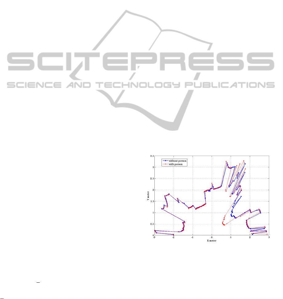
The effect of changing δ values on the observation
model likelihood function peaks was analyzed and
demonstrated using real data recorded from SICK
LMS laser scanner mounted over Pioneer 3AT robot.
The robot position was fixed during this test. The
robot situated inside normal office environment. The
data recorded with and without moving person in the
field of view see Fig.2 . To analyze the peaks, the
Figure 2: Laser scan in typical office environment.
likelihood function has been calculated between each
scan and the whole data set. Fig.3 shows the ratio be-
tween the first to the second peaks in the likelihood
function for all the recorded scans. Again, the robot
position is fixed so ideally there should be no domi-
nant peaks since the pose is not changing. The only
change is in the moving person position and the mea-
surement noise. It is clear that larger values of δ result
AnImprovementintheObservationModelforMonteCarloLocalization
501
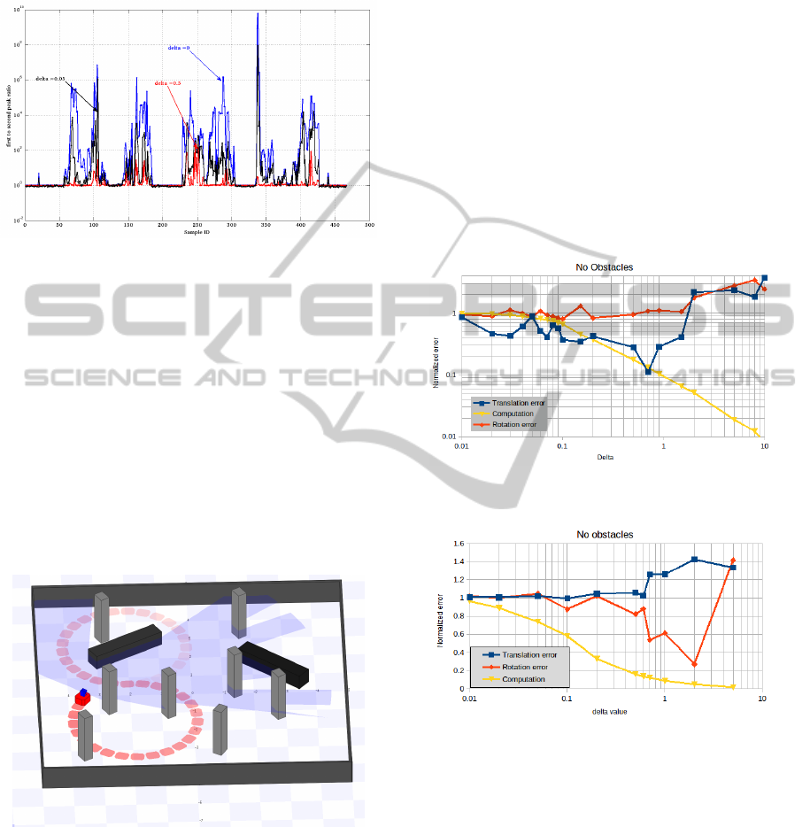
in less dominant peaks. The segments with no peaks
in the figure represents the scans recorded when the
moving person is out of the scanner field of view.
Figure 3: First to second peak ratio in likelihood function
for δ = 0,0.0.5 and 0.5; blue black red respectively .
The described reduction scheme has been verified
using Robot Operating System (ROS) fuerte release
(Willow Garage, 2012) and stage simulator (Vaughan,
2008). The standard ROS monte-carlo localization al-
gorithm (amcl) has been used with modifications in
the observation model. The global localization has
been used in all simulations. The initial robot posi-
tion is assumed to be unknown. The robot moves in
two paths, the first path is 8 shape path while the sec-
ond one is c shaped path. The robot is assumed to
operate inside a small room with only two fixed rect-
angular obstacles and 8 umodeled obstacles see Fig.
4.
Figure 4: simple room with 2 modeled obstacles (black) and
8 extra unmodeled obstacles (gray).
A map of this environment with only two fixed ob-
stacles was build using the slam gmapping node in
ROS with resolution 0.050 m/pix. The robot transla-
tion speed was set to 1m/s. The number of particles
was fixed to 1200 particles. The simulations divided
into three groups:
6.1 No Extra Obstacles
Fig 5 shows the results obtained from the 8 shape path
and no extra obstacles case. It is clear from the blue
line that for δ values less than 1, the translation er-
ror is reduced as delta is increased. A δ value around
0.7 is giving the best combination between transla-
tion error and computation. All the measurements are
normalized with the values obtained from the original
monte-carlo localization algorithm (i.e. the case that
δ = 0). The blue line is the normalized translation er-
ror, the red line is the normalized rotational error and
the yellow line is the normalized computation reduc-
tion.
Fig 6 shows the same case but with C shape path.
Figure 5: Normalized translation error, rotation error and
computations versus δ value with no extra obstacles.
Figure 6: Normalized translation error, rotation error and
computations versus δ value with no extra obstacles .
6.2 Extra Stationary Obstacles
Fig 7 shows the results obtained from the 8 shape path
with extra obstacles case. Fig 8 shows the same case
but with C shape path.
6.3 Extra Moving Obstacles
Fig 9 shows the results obtained from the 8 shape path
with extra moving obstacles case. Fig 10 shows the
same case but with C shape path.
ICINCO2014-11thInternationalConferenceonInformaticsinControl,AutomationandRobotics
502
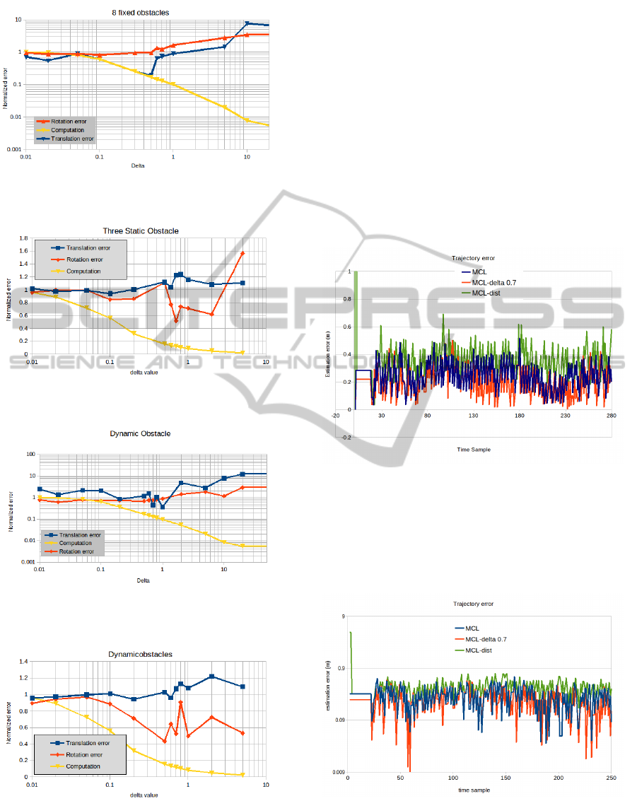
Figure 7: Normalized translation error, rotation error and
computations versus δ value with 8 extra obstacles.
Figure 8: Normalized translation error, rotation error and
computations versus δ value with 8 extra obstacles.
Figure 9: Normalized translation error, rotation error and
computations versus δ value with moving obstacles.
Figure 10: Normalized translation error, rotation error and
computations versus δ value with moving obstacles.
It is clear from all the figures above that applying
this simple reduction scheme results in a noticeable
improvement either in the translation error or in the
rotational error beside approximately 50% reduction
in computation complexity.
6.4 Trajectory Error
To investigate the performance of the proposed algo-
rithm the trajectory error for three different cases is
shown below. The trajectory error is computed as
the difference between the position estimation and the
ground truth for each time sample. In each case a
comparison with the standard MCL and MCL with
distance filter proposed by (Burgard and Thrun, 1999)
is presented.
Figure 11: Trajectory error comparison for no obstacles
case.
Fig. 11 shows the case where no unmodeled ob-
stacles is presented. The estimation error for the pro-
posed algorithm is clearly lower than the others. Also
it is clear that the MCL with distance filter has higher
estimation error.
Figure 12: Trajectory error comparison for moving obsta-
cles case.
Fig. 12 shows the case where dynamic obstacles are
presented in the environment. Again the estimation
error for the proposed algorithm is clearly lower than
AnImprovementintheObservationModelforMonteCarloLocalization
503
the others and the MCL with distance filter has higher
estimation error.
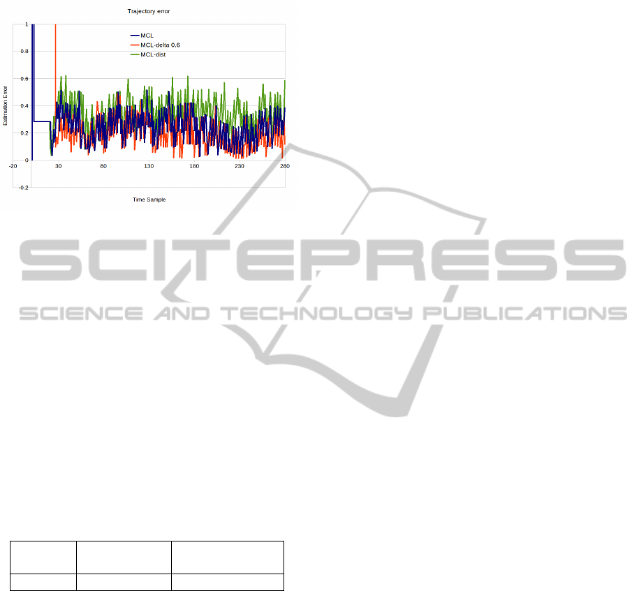
Figure 13: Trajectory error comparison for static obstacles
case.
Fig. 13 shows the case where static but unmod-
eled obstacles are presented in the environment. In
this case also the estimation error for the proposed al-
gorithm is clearly lower than the others and the MCL
with distance filter has higher estimation error.
6.5 Computation Complexity
The Table below shows the computation complexity
of the proposed technique compared with traditional
MCL and MCL with distance filter. It is very clear
that there is a very large reduction in computations.
The number represents how frequent the ray casting
function is called. It is normalized to standard MCL
value. The δ value was set to 0.7 in this table.
Table 1: Computation Complexity reduction table.
Standard MCL with MCL with
MCL Distance filter proposed scheme
1 1.994 0.12832
7 CONCLUSION AND FUTURE
WORK
In this research a modification to observation model
that is used in Monte Carlo localization has been pro-
posed. This modification reduces the peaks generated
in the observation likelihood function that is limiting
the performance of the localization process. Specif-
ically the peaks generated due to the invalidation of
the independent noise assumption between different
measurement beams.
The proposed scheme has been verified using Stage
simulator and ROS Robot operating system. the re-
sults shows improvement in both location estimation
error and the computations required for localization.
As future work, it is possible to find a reliable method
to calculate or estimate the conditional probabilities
in Eq.12 instead of neglecting some measurements.
Also it is important to find solutions to other causes
of the peaks in the observation model. This will defi-
nitely improves the localization farther.
REFERENCES
Burgard, W. and Thrun, S. (1999). Markov localization
for mobile robots in dynamic environments dieter fox
dfox@ cs. cmu. edu computer science department and
robotics institute carnegie mellon university. Journal
of Artificial Intelligence Research, 11:391–427.
Dellaert, F., Fox, D., Burgard, W., and Thrun, S. (1999).
Monte carlo localization for mobile robots. In
Robotics and Automation, 1999. Proceedings. 1999
IEEE International Conference on, volume 2, pages
1322–1328. IEEE.
Fox, D., Burgard, W., Dellaert, F., and Thrun, S. (1999).
Monte carlo localization: Efficient position estimation
for mobile robots. AAAI/IAAI, 1999:343–349.
Olufs, S. and Vincze, M. (2009). An efficient area-based
observation model for monte-carlo robot localization.
In Intelligent Robots and Systems, 2009. IROS 2009.
IEEE/RSJ International Conference on, pages 13–20.
IEEE.
Pfaff, P., Burgard, W., and Fox, D. (2006). Robust monte-
carlo localization using adaptive likelihood models. In
European robotics symposium 2006, pages 181–194.
Springer.
Pfaff, P., Plagemann, C., and Burgard, W. (2007). Improved
likelihood models for probabilistic localization based
on range scans. In Intelligent Robots and Systems,
2007. IROS 2007. IEEE/RSJ International Conference
on, pages 2192–2197. IEEE.
Pfaff, P., Plagemann, C., and Burgard, W. (2008a). Gaus-
sian mixture models for probabilistic localization. In
Robotics and Automation, 2008. ICRA 2008. IEEE In-
ternational Conference on, pages 467–472. IEEE.
Pfaff, P., Stachniss, C., Plagemann, C., and Burgard, W.
(2008b). Efficiently learning high-dimensional ob-
servation models for monte-carlo localization using
gaussian mixtures. In Intelligent Robots and Systems,
2008. IROS 2008. IEEE/RSJ International Conference
on, pages 3539–3544. IEEE.
Plagemann, C., Kersting, K., Pfaff, P., and Burgard, W.
(2007). Gaussian beam processes: A nonparametric
bayesian measurement model for range finders. In
Robotics: Science and Systems.
Rowekamper, J., Sprunk, C., Tipaldi, G. D., Stachniss, C.,
Pfaff, P., and Burgard, W. (2012). On the position
accuracy of mobile robot localization based on parti-
cle filters combined with scan matching. In Intelligent
Robots and Systems (IROS), 2012 IEEE/RSJ Interna-
tional Conference on, pages 3158–3164. IEEE.
ICINCO2014-11thInternationalConferenceonInformaticsinControl,AutomationandRobotics
504

Thrun, S., Burgard, W., and Fox, D. (2005). Probabilistic
robotics. MIT press.
Thrun, S., Fox, D., Burgard, W., and Dellaert, F. (2001).
Robust monte carlo localization for mobile robots. Ar-
tificial Intelligence, 128(1):99–141.
Vaughan, R. (2008). Massively multi-robot simulation in
stage.
Willow Garage, S. A. I. L. (2012). The robot operating
system.
Yilmaz, S., Kayir, H. E., Kaleci, B., and Parlaktuna, O.
(2010). A new sensor model for particle-filter based
localization in the partially unknown environments. In
Systems Man and Cybernetics (SMC), 2010 IEEE In-
ternational Conference on, pages 428–434. IEEE.
AnImprovementintheObservationModelforMonteCarloLocalization
505
